Unit Weibull distribution

Unit Weibull
Probability density function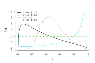
Cumulative distribution function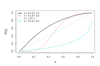
Parameters	${\displaystyle \alpha >0\,}$ (real) ${\displaystyle \beta >0\,}$ (real)
Support	${\displaystyle x\in (0,1)\,}$
PDF	${\displaystyle {\frac {1}{x}}\,\alpha \,\beta \,(-\log x)^{\beta -1}\exp \left[-\alpha \,(-\log x)^{\beta }\right]}$
CDF	${\displaystyle \exp \left[-\alpha \,(-\log x)^{\beta }\right]}$
Quantile	${\displaystyle \exp \left[-\left({\frac {-\log p}{\alpha }}\right)^{\frac {1}{\beta }}\right],\quad 0<p<1}$
Skewness	${\displaystyle {\frac {\mu '_{3}-3\mu '_{2}\mu +\mu ^{3}}{\sigma ^{3}}}}$
Excess kurtosis	${\displaystyle {\frac {\mu '_{4}-4\mu '_{3}\mu +6\mu '_{2}\mu ^{2}-3\mu ^{4}}{\sigma ^{4}}}}$
MGF	${\displaystyle \sum _{n=0}^{\infty }{\frac {(-1)^{n}}{n!\,\alpha ^{n/\beta }}}\,\Gamma \left({\frac {n}{\beta }}+1\right)}$

The unit-Weibull distribution (UW) is a continuous probability distribution with domain on ${\displaystyle (0,1)}$. Useful for indices and rates, or bounded variables with a ${\displaystyle (0,1)}$ domain. It was originally proposed by Mazucheli et al¹ using a transformation of the Weibull distribution.

Its probability density function is defined as:

${\displaystyle f(x;\alpha ,\beta )={\frac {1}{x}}\,\alpha \,\beta \,(-\log x)^{\beta -1}\exp \left[-\alpha \,(-\log x)^{\beta }\right]}$

And its cumulative distribution function is:

${\displaystyle F(x;\alpha ,\beta )=\exp \left[-\alpha \,(-\log x)^{\beta }\right]}$

The quantile function of the UW distribution is given by:

${\displaystyle Q(p)=\exp \left[-\left({\frac {-\log p}{\alpha }}\right)^{\frac {1}{\beta }}\right],\quad 0<p<1.}$

Having a closed form expression for the quantile function, may make it a more flexible alternative for a quantile regression model against the classical Beta regression model.

The ${\displaystyle r}$th raw moment of the UW distribution can be obtained through:

${\displaystyle \mu '_{r}=\mathbb {E} (X^{r})=\mathbb {E} (e^{-rY})=M_{Y}(-r)=\sum _{n=0}^{\infty }{\frac {(-1)^{n}}{n!\,\alpha ^{n/\beta }}}\,\Gamma \left({\frac {n}{\beta }}+1\right).}$

The skewness and kurtosis measures can be obtained upon substituting the raw moments from the expressions:

${\displaystyle {\mathit {skewness}}={\frac {\mu '_{3}-3\mu '_{2}\mu +\mu ^{3}}{\sigma ^{3}}},{\mathit {kurtosis}}={\frac {\mu '_{4}-4\mu '_{3}\mu +6\mu '_{2}\mu ^{2}-3\mu ^{4}}{\sigma ^{4}}}}$

The hazard rate function of the UW distribution is given by:

${\displaystyle h(x;\alpha ,\beta )={\frac {f(x;\alpha ,\beta )}{1-F(x;\alpha ,\beta )}}={\frac {\alpha \beta \,(-\log x)^{\beta -1}\exp \left[-\alpha (-\log x)^{\beta }\right]}{x\left(1-\exp \left[-\alpha (-\log x)^{\beta }\right]\right)}},\quad 0<x<1.}$

Let ${\displaystyle \mathbf {x} =(x_{1},\ldots ,x_{n})}$ be a random sample of size ${\displaystyle n}$ from the UW distribution with probability density function defined before. Then, the log-likelihood function of ${\displaystyle {\boldsymbol {\theta }}=(\alpha ,\beta )}$ is:

${\displaystyle {\begin{aligned}\ell ({\boldsymbol {\theta }};\mathbf {x} )&=n(\log \alpha +\log \beta )-\sum _{i=1}^{n}\log x_{i}+(\beta -1)\sum _{i=1}^{n}\log(-\log x_{i})-\alpha \sum _{i=1}^{n}(-\log x_{i})^{\beta }\end{aligned}}}$

The likelihood estimate ${\displaystyle {\hat {\boldsymbol {\theta }}}}$ of ${\displaystyle {\boldsymbol {\theta }}}$ is obtained by solving the non-linear equations

${\displaystyle {\frac {\partial \ell }{\partial \alpha }}={\frac {n}{\alpha }}-\sum _{i=1}^{n}(-\log x_{i})^{\beta }=0,}$

and

${\displaystyle {\frac {\partial \ell }{\partial \beta }}={\frac {n}{\beta }}+\sum _{i=1}^{n}\log(-\log x_{i})-\alpha \sum _{i=1}^{n}(-\log x_{i})^{\beta }\log(-\log x_{i})=0.}$

The expected Fisher information matrix of ${\displaystyle {\boldsymbol {\theta }}=(\alpha ,\beta )}$ based on a single observation is given by

${\displaystyle \mathbf {I} ({\boldsymbol {\theta }})=[I_{ij}]={\begin{pmatrix}{\frac {1}{\alpha }}&{\frac {1}{\alpha \beta }}(1-\gamma -\log \alpha )\\{\frac {1}{\alpha \beta }}(1-\gamma -\log \alpha )&{\frac {1}{\beta ^{2}}}\left[{\frac {\pi ^{2}}{6}}+(1-\gamma -\log \alpha )^{2}\right]\end{pmatrix}},}$

where ${\displaystyle \pi \simeq 3.141593}$ and ${\displaystyle \gamma \simeq 0.577216}$ is the Euler’s constant.

When ${\displaystyle \beta =1}$, ${\displaystyle x}$ follows the power function distribution and the ${\displaystyle r}$th raw moment of the UW distribution becomes:

${\displaystyle \mu '_{r}=\mathbb {E} (X^{r})={\frac {\alpha }{r+\alpha }},\quad r=1,2,\ldots .}$

In this case, the mean, variance, skewness and kurtosis, are:

${\displaystyle \mu ={\frac {\alpha }{1+\alpha }},\qquad \sigma ^{2}={\frac {\alpha }{(1+\alpha )^{2}(2+\alpha )}},}$

${\displaystyle {\textit {skewness}}={\frac {2(1-\alpha )}{(2+\alpha )}}{\sqrt {1+{\frac {2}{\alpha }}}},\qquad {\textit {kurtosis}}={\frac {3(2+\alpha )(2-\alpha +3\alpha ^{2})}{\alpha (3+\alpha )(4+\alpha )}}.}$

The skewness can be negative, zero, or positive when ${\displaystyle \alpha <1,\alpha =1,\alpha >1}$. And if ${\displaystyle \alpha =1}$, with ${\displaystyle \beta =1}$, ${\displaystyle x}$ follows the standard uniform distribution, and the measures becomes:

${\displaystyle \mu ={\frac {1}{2}},\qquad \sigma ^{2}={\frac {1}{12}},\qquad {\textit {skewness}}=0,\quad {\textit {kurtosis}}={\frac {9}{5}}.}$

For the case of ${\displaystyle \beta =2}$, ${\displaystyle x}$ follows the unit-Rayleigh distribution, and:

${\displaystyle \mu '_{r}=\mathbb {E} (X^{r})=1-{\frac {\sqrt {\pi }}{2{\sqrt {\alpha }}}}\,r\,e^{r^{2}/(4\alpha )}\,\mathrm {erfc} \left({\frac {r}{2{\sqrt {\alpha }}}}\right),\qquad r=1,2,\ldots ,}$

where

${\displaystyle \mathrm {erfc} (z)={\frac {2}{\sqrt {\pi }}}\int _{z}^{\infty }e^{-x^{2}}\,dx,\qquad z>0,}$

Is the complementary error function. In this case, the measures of the distribution are:

${\displaystyle \mu =1-{\frac {\sqrt {\pi }}{2{\sqrt {\alpha }}}}\,e^{1/\alpha }\,\mathrm {erfc} \left({\frac {1}{2{\sqrt {\alpha }}}}\right),\sigma ^{2}=1-{\frac {\sqrt {\pi }}{\sqrt {\alpha }}}\,e^{1/\alpha }\,\mathrm {erfc} \left({\frac {1}{\sqrt {\alpha }}}\right)-\left[1-{\frac {\sqrt {\pi }}{2{\sqrt {\alpha }}}}\,e^{1/\alpha }\,\mathrm {erfc} \left({\frac {1}{2{\sqrt {\alpha }}}}\right)\right]^{2}.}$

It was shown to outperform, against other distributions, like the Beta and Kumaraswamy distributions, in: maximum flood level, petroleum reservoirs, risk management cost effectiveness,² and recovery rate of CD34+cells data.