In mathematics, the derivative of a function at a point is the linear part of the best affine approximation to the function near the point. In one-variable calculus, this is the tangent line approximation. In multivariable calculus, the same property is generalized to define the derivative of a vector-valued function or function of a vector argument. Sometimes called the total derivative, in contrast with partial derivatives, the derivative approximates the function with respect to all of its arguments, not just a single one.1 In many situations, this is the same as considering all partial derivatives simultaneously.
In functional analysis, particularly in infinite dimensions, the derivative in this sense is called the Fréchet derivative.23
Derivative as a linear map
Let be an open subset. Then a function is said to be differentiable at a point if there exists a linear transformation such that45
where denotes the norm of . The linear map is called the derivative or differential of at .46 Here refers to applying the linear transformation to the vector ; in coordinates, this is a matrix-vector product. Other notations for the derivative include and . A function is differentiable if its derivative exists at every point in its domain.
Conceptually, the definition of the derivative expresses the idea that is the best linear approximation to for small . This can be made precise by quantifying the error in the linear approximation . To do so, write
where equals the error in the approximation. To say that the derivative of at is is equivalent to the statement
where is little-o notation and means that tends to zero as . The derivative is the unique linear transformation for which the error term is this small, and this is the sense in which it is the best linear approximation to .
Differentiability
The function is differentiable if and only if each of its components is differentiable, so when studying derivatives, it is often possible to work one coordinate at a time in the codomain. However, the same is not true of the coordinates in the domain. It is true that if is differentiable at , then each partial derivative exists at .7
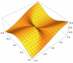
The converse does not hold: it can happen that all of the partial derivatives of at exist, but is not differentiable at .8 An example is the following function, which is continuous and has both partial derivatives zero at the origin, but is not differentiable there: (In polar coordinates, this function is .)
Even the existence and linearity of all directional derivatives at a point is not sufficient for differentiability; the essential additional requirement is that the linear approximation hold uniformly as the increment tends to zero from all directions. An example is whose directional derivatives are all 0 at (0,0), but which fails to be differentiable there.
However, if all the partial derivatives of at exist in a neighborhood of and are continuous at , then is differentiable at .9 If is differentiable at a point, then the derivative of is the linear transformation corresponding to the Jacobian matrix of partial derivatives at the point.10
Differentials
In some advanced calculus texts, the derivative is also called the differential.16 However, this term has several different, but closely connected meanings, in mathematics and the sciences.
When a differentiable function is scalar valued, the derivative of at may be written as the Jacobian matrix, which in this instance is a row matrix (a matrix consisting of elements in a single row, i.e., a row vector):
The linear approximation property of the derivative implies that if
is a small vector (where the denotes transpose, so that this vector is a column vector), then
Heuristically, this suggests that if are infinitesimal increments in the coordinate directions, then
and this is the differential of at .1112 In fact, the notion of the infinitesimal, which is merely symbolic here, can be equipped with extensive mathematical structure. Techniques, such as the theory of differential forms, effectively give analytical and algebraic descriptions of objects like infinitesimal increments, . For instance, may be inscribed as a linear functional on the vector space . Evaluating at a vector in measures how much points in the -th coordinate direction. The differential is a linear combination of linear functionals and hence is itself a linear functional. The evaluation is the directional derivative of along . This point of view makes the derivative an instance of the exterior derivative.13
Being a linear form, the differential is naturally a covector. In a Euclidean space, a covector is naturally dual to a vector (its transpose). This vector is called the gradient of , and points in the direction in which increases most rapidly.
Suppose now that is a vector-valued function, that is, . In this case, the components of are real-valued functions, so they have associated differential forms . The differential amalgamates these forms into a single object and is therefore an instance of a vector-valued differential form.
If is a mapping between differentiable manifolds, differentiability can be formulated by differentiability in any coordinate chart. Invariantly, the differential of at a point is a linear map from the tangent space of at to that of at .1415 This is also known as the pushforward. This is closely related to the derivative as a linear approximation, since evaluating on a tangent vector gives the directional derivative of in that direction. Nevertheless, the differential is not quite the same thing as the derivative of a function between vector spaces: is a mapping of manifolds and not of the vector spaces and where the linear approximation lives.
In applications such as thermodynamics, the language of differentials often has an additional conceptual role. Expressions such as describe differentials of state functions and lead to questions about exactness, natural variables, and relations among partial derivatives. This use is related to the derivative of a multivariable function, but it is not just another name for the linear map associated with an ordinary function.1617
Total derivative
The term total derivative is also used in more than one way. In some mathematical texts it denotes the full derivative , as opposed to any one partial derivative. In that sense, the total derivative is the linear map that accounts for variation in all coordinate directions simultaneously.
In many applied contexts, however, "total derivative" refers instead to the derivative of a composite dependence. For example, if
then the total derivative of with respect to is
This is the ordinary derivative of the composite function , computed by the chain rule. Equivalently, it is obtained by applying the derivative of to the velocity vector of the path :
This chain-rule sense of "total derivative" is common in physics, engineering, economics, and other applied fields. In mechanics, for instance, the total time derivative of a function along a trajectory includes both explicit dependence on and implicit dependence through the time-dependent variables and . In fluid mechanics, related terminology appears in the material derivative, which differentiates a quantity along the motion of a fluid parcel.1819
Another example is in classical mechanics, where the total derivative of a function that depends on phase space parameters and time is its partial derivative in time plus its Poisson bracket with the Hamiltonian :20 Like the material derivative, total derivative in mechanics has the property that it is the derivative of the composite when pulled back to any Hamiltonian trajectory, but is still treated as a function of all phase space coordinates and time.
In comparative statics, total derivatives often describe how endogenous variables change with respect to exogenous variables in an implicitly defined system of equations.21 The endogeneous variables are generally not explicit functions of the exogeneous variables, other than through the implicit function theorem, and the total derivative is handled implicitly.
Thus, although "total derivative" can mean the derivative in the sense above, the term also commonly refers to a derivative along a specified dependence or process. This ambiguity is one reason to distinguish between the derivative as a linear map and the various differential or total-derivative notations used in applications.
Chain rule
A form of the chain rule generalizes from one-variable calculus. It says that, for two functions and , the derivative of the composite function at satisfies
where the composite on the right-hand side is the composition of linear maps. If the derivatives of and are identified with their Jacobian matrices, then the composite on the right-hand side is simply matrix multiplication.
Example: Differentiation with direct dependencies
Suppose that f is a function of two variables, x and y. If these two variables are independent, so that the domain of f is , then the behavior of f may be understood in terms of its partial derivatives in the x and y directions. However, in some situations, x and y may be dependent. For example, it might happen that f is constrained to a curve . In this case, we are actually interested in the behavior of the composite function . The partial derivative of f with respect to x does not give the true rate of change of f with respect to changing x because changing x necessarily changes y, while the partial derivative assumes y is fixed. However, the chain rule takes such dependencies into account. Write . Then, the chain rule says
By expressing the derivative using Jacobian matrices such asThis becomes:
Suppressing the evaluation at for legibility, we may also write this as
This gives a straightforward formula for the derivative of in terms of the partial derivatives of and the derivative of .
For example, suppose
The rate of change of f with respect to x is usually the partial derivative of f with respect to x; in this case,
However, if y depends on x, the partial derivative does not give the true rate of change of f as x changes because the partial derivative assumes that y is fixed. Suppose we are constrained to the line
Then
and the total derivative of f with respect to x is
which we see is not equal to the partial derivative . Instead of immediately substituting for y in terms of x, however, we can also use the chain rule as above:
Example: Differentiation with indirect dependencies
While one can often perform substitutions to eliminate indirect dependencies, the chain rule provides for a more efficient and general technique. Suppose is a function of time and variables which themselves depend on time. Then, the time derivative of is
The chain rule expresses this derivative in terms of the partial derivatives of and the time derivatives of the functions :
This expression is often used in physics for a gauge transformation of the Lagrangian, as two Lagrangians that differ only by the total time derivative of a function of time and the generalized coordinates lead to the same equations of motion. An interesting example concerns the resolution of causality concerning the Wheeler–Feynman time-symmetric theory. The operator in brackets (in the final expression above) is also called the total derivative operator (with respect to ).
For example, the total derivative of is
Here there is no term since itself does not depend on the independent variable directly.
Total differential equation
A total differential equation is a differential equation expressed in terms of total derivatives. Since the exterior derivative is coordinate-free, in a sense that can be given a technical meaning, such equations are intrinsic and geometric.
Application to equation systems
In economics, it is common for the total derivative to arise in the context of a system of equations.22: pp. 217–220 For example, a simple supply-demand system might specify the quantity q of a product demanded as a function D of its price p and consumers' income I, the latter being an exogenous variable, and might specify the quantity supplied by producers as a function S of its price and two exogenous resource cost variables r and w. The resulting system of equations
determines the market equilibrium values of the variables p and q. The total derivative of p with respect to r, for example, gives the sign and magnitude of the reaction of the market price to the exogenous variable r. In the indicated system, there are a total of six possible total derivatives, also known in this context as comparative static derivatives: dp/dr, dp/dw, dp/dI, dq/dr, dq/dw, and dq/dI. The total derivatives are found by totally differentiating the system of equations, dividing through by, say dr, treating dq/dr and dp/dr as the unknowns, setting dI = dw = 0, and solving the two totally differentiated equations simultaneously, typically by using Cramer's rule.
See also
See also
- Directional derivative – Instantaneous rate of change of the function
- Fréchet derivative – Derivative defined on normed spaces - generalization of the total derivative
- Functional derivative – Concept in calculus of variations
- Gateaux derivative – Generalization of the concept of directional derivative
- Generalizations of the derivative – Fundamental construction of differential calculus
- Gradient#Total derivative – Multivariate derivative (mathematics)
References
References
- Rudin 1976, p. 213.
- Lang 1987, §XIII.3.
- Abraham, Marsden & Ratiu 1988, pp. 76–78.
- Rudin 1976, pp. 212–214.
- Munkres 1991, pp. 34–36.
- Spivak 1965, pp. 14–15.
- Rudin 1976, pp. 215–216.
- Munkres 1991, pp. 48–50.
- Apostol 1981, Theorem 12.11.
- Abraham, Marsden & Ratiu 1988, p. 78.
- Spivak 1965, pp. 89–91.
- Lee 2013, p. 74.
- Lee 2013, pp. 276–279.
- Lee 2013, pp. 65–68.
- Tu 2011, pp. 82–86.
- Callen 1985, pp. 35–38.
- Zemansky & Dittman 1997.
- Batchelor 1967, p. 73.
- White 2011, pp. 138–140.
- Arnold 1989.
- Chiang 1984, Section 8.6. sfn error: multiple targets (2×): CITEREFChiang1984 (help)
- Chiang, Alpha C. (1984). Fundamental Methods of Mathematical Economics (Third ed.). McGraw-Hill. ISBN 0-07-010813-7.
- Abraham, Ralph; Marsden, Jerrold E.; Ratiu, Tudor (1988), Manifolds, Tensor Analysis, and Applications (2nd ed.), Springer, ISBN 978-0-387-96790-5.
- Apostol, Tom M. (1981), Calculus, Volume II: Multi-Variable Calculus and Linear Algebra, with Applications to Differential Equations and Probability (2nd ed.), John Wiley & Sons, ISBN 978-0-471-00007-5.
- Arnold, Vladimir I. (1989), Mathematical Methods of Classical Mechanics, translated by Vogtmann, K. (2nd ed.), Springer, ISBN 978-0-387-96890-2.
- Batchelor, G. K. (1967), An Introduction to Fluid Dynamics, Cambridge University Press, ISBN 978-0-521-66396-0.
- Callen, Herbert B. (1985), Thermodynamics and an Introduction to Thermostatistics (2nd ed.), John Wiley & Sons, ISBN 978-0-471-86256-7.
- Chiang, Alpha C. (1984), Fundamental Methods of Mathematical Economics (3rd ed.), McGraw-Hill, ISBN 0-07-010813-7.
- Goldstein, Herbert; Poole, Charles P.; Safko, John L. (2002), Classical Mechanics (3rd ed.), Addison-Wesley, ISBN 978-0-201-65702-9.
- Lang, Serge (1987), Calculus of Several Variables (3rd ed.), Springer.
- Lee, John M. (2013), Introduction to Smooth Manifolds, Graduate Texts in Mathematics, vol. 218 (2nd ed.), Springer, ISBN 978-1-4419-9981-8.
- Loomis, Lynn H.; Sternberg, Shlomo (1990), Advanced Calculus (Revised ed.), Jones and Bartlett, ISBN 978-0-86720-122-2.
- Munkres, James R. (1991), Analysis on Manifolds, Addison-Wesley, ISBN 978-0-201-51035-5.
- Polyanin, Andrei D.; Zaitsev, Valentin F. (2003), Handbook of Exact Solutions for Ordinary Differential Equations (2nd ed.), Chapman & Hall/CRC, ISBN 1-58488-297-2.
- Rudin, Walter (1976), Principles of Mathematical Analysis (3rd ed.), McGraw-Hill, ISBN 007054235X.
- Spivak, Michael (1965), Calculus on Manifolds: A Modern Approach to Classical Theorems of Advanced Calculus, W. A. Benjamin, ISBN 978-0-8053-9021-6.
- Tu, Loring W. (2011), An Introduction to Manifolds, Universitext (2nd ed.), Springer, ISBN 978-1-4419-7399-3.
- White, Frank M. (2011), Fluid Mechanics (7th ed.), McGraw-Hill, ISBN 978-0-07-352934-9.
- Zemansky, Mark W.; Dittman, Richard H. (1997), Heat and Thermodynamics (7th ed.), McGraw-Hill, ISBN 978-0-07-017059-9.
- A. D. Polyanin and V. F. Zaitsev, Handbook of Exact Solutions for Ordinary Differential Equations (2nd edition), Chapman & Hall/CRC Press, Boca Raton, 2003. ISBN 1-58488-297-2
- From thesaurus.maths.org total derivative