Article · Wikipedia archive·Last revised Jun 6, 2026
Rectangular mask short-time Fourier transform
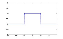
In mathematics and Fourier analysis, a rectangular mask short-time Fourier transform (rec-STFT) is a simplified form of the short-time Fourier transform which is used to analyze how a signal's frequency content changes over time. In rec-STFT, a rectangular window is used to isolate short time segments of the signal. Other types of the STFT may require more computation time than the rec-STFT.
In mathematics and Fourier analysis, a rectangular mask short-time Fourier transform (rec-STFT) is a simplified form of the short-time Fourier transform which is used to analyze how a signal's frequency content changes over time. In rec-STFT, a rectangular window (a simple on/off time-limiting function) is used to isolate short time segments of the signal. Other types of the STFT may require more computation time ( refers to the amount of time it takes a computer or algorithm to perform a calculation or complete a task) than the rec-STFT.
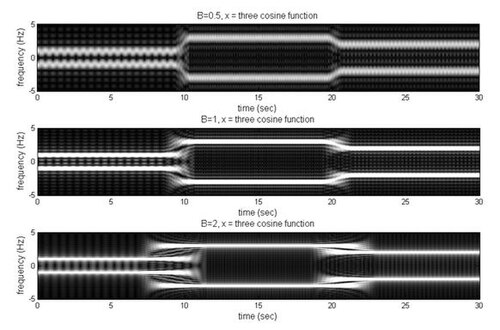
Spectrograms produced from applying a rec-STFT on a function consisting of 3 consecutive cosine waves. (top spectrogram uses smaller B of 0.5, middle uses B of 1, and bottom uses larger B of 2.) source ↗
From the image, when B is smaller, the time resolution is better. Otherwise, when B is larger, the frequency resolution is better.
Advantage and disadvantage
Compared with the Fourier transform:
Advantage: The instantaneous frequency can be observed.
Advantage: Least computation time for digital implementation.
Disadvantage: Quality is worse than other types of time-frequency analysis. The jump discontinuity of the edges of the rectangular mask results in Gibbs ringing artifacts in the frequency domain, which can be alleviated with smoother windows.