Reciprocal distribution

Reciprocal
Probability density function
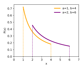
Cumulative distribution function
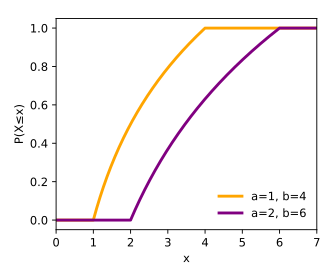
Parameters	${\displaystyle 0<a<b,a,b\in \mathbb {R} }$
Support	${\displaystyle [a,b]}$
PDF	${\displaystyle {\frac {1}{x\ln {\frac {b}{a}}}}}$
CDF	${\displaystyle {\frac {\ln {\frac {x}{a}}}{\ln {\frac {b}{a}}}}}$
Mean	${\displaystyle {\frac {b-a}{\ln {\frac {b}{a}}}}}$
Median	${\displaystyle {\sqrt {ab}}}$
Mode	${\displaystyle a}$
Variance	${\displaystyle {\frac {b^{2}-a^{2}}{2\ln {\frac {b}{a}}}}-\left({\frac {b-a}{\ln {\frac {b}{a}}}}\right)^{2}}$
Entropy	${\displaystyle \ln \left(\ln \left({\frac {b}{a}}\right)\right)+{\frac {\ln \left(b\right)^{2}-\ln \left(a\right)^{2}}{2\ln \left({\frac {b}{a}}\right)}}}$
MGF	${\displaystyle {\frac {{\rm {Ei}}(bt)-{\rm {Ei}}(at)}{\ln \left(b\right)-\ln \left(a\right)}}}$
CF	${\displaystyle {\frac {{\rm {Ei}}(ibt)-{\rm {Ei}}(iat)}{\ln \left(b\right)-\ln \left(a\right)}}}$

In probability and statistics, the reciprocal distribution, also known as the log-uniform distribution, is a continuous probability distribution. It is characterised by its probability density function, within the support of the distribution, being proportional to the reciprocal of the variable.

The reciprocal distribution is an example of an inverse distribution, and the reciprocal (inverse) of a random variable with a reciprocal distribution itself has a reciprocal distribution.

The probability density function (pdf) of the reciprocal distribution is

${\displaystyle f(x;a,b)={\frac {1}{x[\ln(b)-\ln(a)]}}\quad {\text{ for }}a\leq x\leq b{\text{ and }}a>0.}$

Here, ${\displaystyle a}$ and ${\displaystyle b}$ are the parameters of the distribution, which are the lower and upper bounds of the support, and ${\displaystyle \ln }$ is the natural log. The cumulative distribution function is

${\displaystyle F(x;a,b)={\frac {\ln(x)-\ln(a)}{\ln(b)-\ln(a)}}\quad {\text{ for }}a\leq x\leq b.}$

A positive random variable X is log-uniformly distributed if the logarithm of X is uniform distributed,

${\displaystyle \ln(X)\sim {\mathcal {U}}(\ln(a),\ln(b)).}$

This relationship is true regardless of the base of the logarithmic or exponential function. If ${\displaystyle \log _{a}(Y)}$ is uniform distributed, then so is ${\displaystyle \log _{b}(Y)}$, for any two positive numbers ${\displaystyle a,b\neq 1}$. Likewise, if ${\displaystyle e^{X}}$ is log-uniform distributed, then so is ${\displaystyle a^{X}}$, where ${\displaystyle 0<a\neq 1}$.

The reciprocal distribution is of considerable importance in numerical analysis, because a computer’s arithmetic operations, in particular, repeated multiplications and/or divisions, transform mantissas with initial arbitrary distributions into the reciprocal distribution as a limiting distribution.¹

References

1. Hamming R. W. (1970) "On the distribution of numbers", The Bell System Technical Journal 49(8) 1609–1625