Article · Wikipedia archive · Last revised May 27, 2026

Power iteration

In mathematics, power iteration is an eigenvalue algorithm: given a diagonalizable matrix , the algorithm will produce a number , which is the greatest eigenvalue of , and a nonzero vector , which is a corresponding eigenvector of , that is, . The algorithm is also known as the Von Mises iteration.

Last revised
May 27, 2026
Read time
≈ 11 min
Length
2,454 w
Citations
4
Source

In mathematics, power iteration (also known as the power method) is an eigenvalue algorithm: given a diagonalizable matrix A {\displaystyle A} , the algorithm will produce a number λ {\displaystyle \lambda } , which is the greatest (in absolute value) eigenvalue of A {\displaystyle A} , and a nonzero vector v {\displaystyle v} , which is a corresponding eigenvector of λ {\displaystyle \lambda } , that is, A v = λ v {\displaystyle Av=\lambda v} . The algorithm is also known as the Von Mises iteration.1

Power iteration is a very simple algorithm, but it may converge slowly. The most time-consuming operation of the algorithm is the multiplication of matrix A {\displaystyle A} by a vector, so it is effective for a very large sparse matrix with appropriate implementation. The speed of convergence is like ( λ 2 / λ 1 ) k {\displaystyle (\lambda _{2}/\lambda _{1})^{k}} where k {\displaystyle k} is the number of iterations, and λ 1 {\displaystyle \lambda _{1}} and λ 2 {\displaystyle \lambda _{2}} are, respectively, the eigenvalue of largest absolute value and an eigenvalue of second-largest absolute value (see a later section). In other words, convergence is exponential with base being the spectral gap.

The method
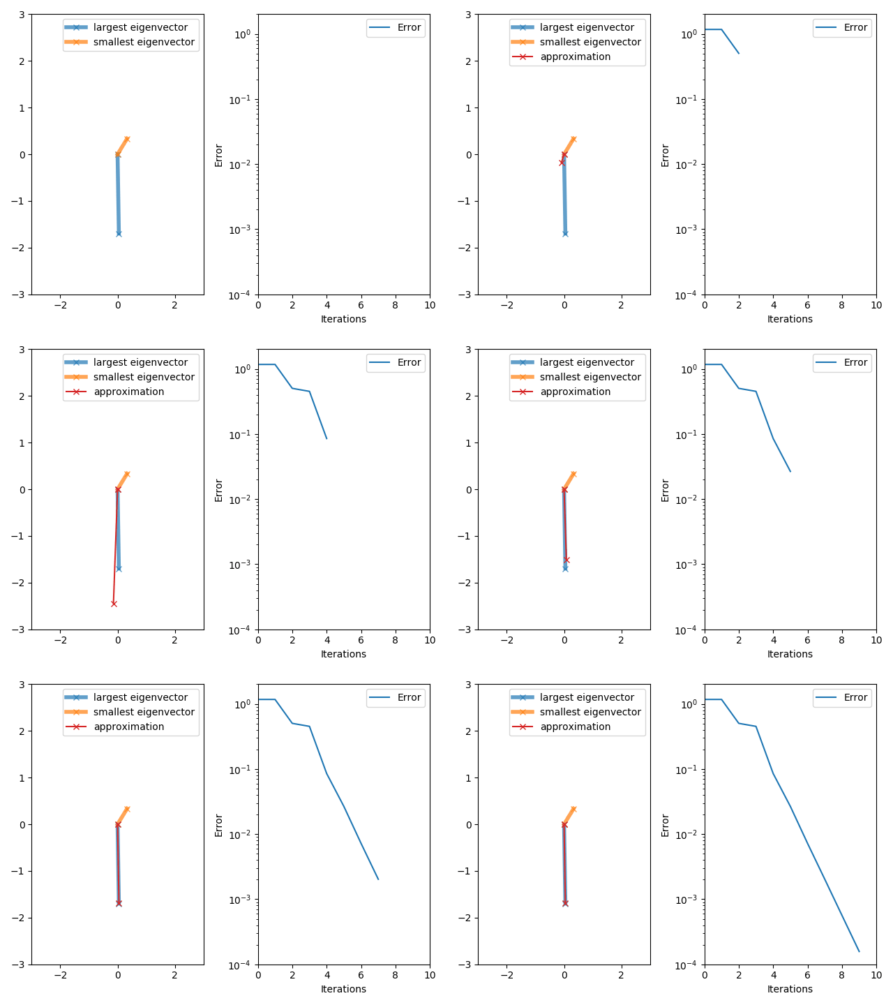
Animation that visualizes the power iteration algorithm on a 2 x 2 matrix. The matrix is depicted by its two eigenvectors. Error is computed as | | approximation largest eigenvector | | {\displaystyle ||{\text{approximation}}-{\text{largest eigenvector}}||} source ↗

The power iteration algorithm starts with a vector b 0 {\displaystyle b_{0}} , which may be an approximation to the dominant eigenvector or a random vector. The method is described by the recurrence relation

b k + 1 = A b k A b k {\displaystyle b_{k+1}={\frac {Ab_{k}}{\lVert Ab_{k}\rVert }}}

So, at every iteration, the vector b k {\displaystyle b_{k}} is multiplied by the matrix A {\displaystyle A} and normalized.

If we assume A {\displaystyle A} has an eigenvalue that is strictly greater in magnitude than its other eigenvalues, i.e.,

| λ 1 | > | λ 2 | | λ n | 0 {\displaystyle \left\vert \lambda _{1}\right\vert >\left\vert \lambda _{2}\right\vert \geq \ldots \geq \left\vert \lambda _{n}\right\vert \geq 0}

and the starting vector b 0 {\displaystyle b_{0}} has a nonzero component in the direction of an eigenvector associated with the dominant eigenvalue, then a subsequence ( b k ) {\displaystyle \left(b_{k}\right)} converges to an eigenvector associated with the dominant eigenvalue.

Without the two assumptions above, the sequence ( b k ) {\displaystyle \left(b_{k}\right)} does not necessarily converge. In this sequence,

b k = e i ϕ k v 1 + r k {\displaystyle b_{k}=e^{i\phi _{k}}v_{1}+r_{k}} ,

where v 1 {\displaystyle v_{1}} is an eigenvector associated with the dominant eigenvalue, and r k 0 {\displaystyle \|r_{k}\|\rightarrow 0} . The presence of the term e i ϕ k {\displaystyle e^{i\phi _{k}}} implies that ( b k ) {\displaystyle \left(b_{k}\right)} does not converge unless e i ϕ k = 1 {\displaystyle e^{i\phi _{k}}=1} . Under the two assumptions listed above, the sequence ( μ k ) {\displaystyle \left(\mu _{k}\right)} defined by

μ k = b k A b k b k b k {\displaystyle \mu _{k}={\frac {b_{k}^{*}Ab_{k}}{b_{k}^{*}b_{k}}}}

converges to the dominant eigenvalue (with Rayleigh quotient).

One may compute this with the following algorithm (shown in Python with NumPy):

import numpy as np
from numpy import typing as npt

def random_vector(dimension: int) -> npt.NDArray[np.float64]:
    rng = np.random.default_rng()
    return rng.random(dimension)

def power_method(
    A: npt.NDArray[np.float64],
    num_iterations: int,
) -> npt.NDArray[np.float64]:
    if A.shape[0] != A.shape[1]:
        raise ValueError("A must be a square matrix.")
    
    # Choose a random initial vector to reduce the chance
    # that it is orthogonal to the dominant eigenvector.
    b_k = random_vector(A.shape[1])

    # Normalize the initial vector.
    b_k /= np.linalg.norm(b_k)

    for _ in range(num_iterations):
        # Multiply by the matrix.
        b_k1 = A @ b_k

        # Compute the length of the new vector.
        b_k1_norm = np.linalg.norm(b_k1)

        # Stop if the new vector is within machine precision of 0.
        if np.isclose(b_k1_norm, 0.0):
            raise ValueError("Power method produced the zero vector.")

        # Normalize the vector for the next iteration.
        b_k = b_k1 / b_k1_norm

    # Return the approximate dominant eigenvector.
    return b_k

The vector b k {\displaystyle b_{k}} converges to an associated eigenvector. Ideally, one should use the Rayleigh quotient in order to get the associated eigenvalue.

This algorithm is used to calculate the Google PageRank.

The method can also be used to calculate the spectral radius (the eigenvalue with the largest magnitude, for a square matrix) by computing the Rayleigh quotient

ρ ( A ) = max { | λ 1 | , | λ 2 | , , | λ n | } = b k A b k b k b k . {\displaystyle \rho (A)=\max \left\{\vert \lambda _{1}\vert ,\vert \lambda _{2}\vert ,\ldots ,\vert \lambda _{n}\vert \right\}={\frac {b_{k}^{\top }Ab_{k}}{b_{k}^{\top }b_{k}}}.}

Analysis

Let A {\displaystyle A} be decomposed into its Jordan canonical form: A = V J V 1 {\displaystyle A=VJV^{-1}} , where the first column of V {\displaystyle V} is an eigenvector of A {\displaystyle A} corresponding to the dominant eigenvalue λ 1 {\displaystyle \lambda _{1}} . Since generically, the dominant eigenvalue of A {\displaystyle A} is unique, the first Jordan block of J {\displaystyle J} is the 1 × 1 {\displaystyle 1\times 1} matrix [ λ 1 ] , {\displaystyle [\lambda _{1}],} where λ 1 {\displaystyle \lambda _{1}} is the largest eigenvalue of A {\displaystyle A} in magnitude. The starting vector b 0 {\displaystyle b_{0}} can be written as a linear combination of the columns of V {\displaystyle V} :

b 0 = c 1 v 1 + c 2 v 2 + + c n v n . {\displaystyle b_{0}=c_{1}v_{1}+c_{2}v_{2}+\ldots +c_{n}v_{n}.}

By assumption, b 0 {\displaystyle b_{0}} has a nonzero component in the direction of the dominant eigenvector, so c 1 0 {\displaystyle c_{1}\neq 0} .

The computationally useful recurrence relation for b k + 1 {\displaystyle b_{k+1}} can be rewritten as:

b k + 1 = A b k A b k = A k + 1 b 0 A k + 1 b 0 , {\displaystyle b_{k+1}={\frac {Ab_{k}}{\|Ab_{k}\|}}={\frac {A^{k+1}b_{0}}{\|A^{k+1}b_{0}\|}},}

where the expression: A k + 1 b 0 A k + 1 b 0 {\displaystyle {\frac {A^{k+1}b_{0}}{\|A^{k+1}b_{0}\|}}} is more amenable to the following analysis:

b k = A k b 0 A k b 0 = ( V J V 1 ) k b 0 ( V J V 1 ) k b 0 (since A is diagonalizable) = V J k V 1 b 0 V J k V 1 b 0 = V J k V 1 ( c 1 v 1 + c 2 v 2 + + c n v n ) V J k V 1 ( c 1 v 1 + c 2 v 2 + + c n v n ) = V J k ( c 1 e 1 + c 2 e 2 + + c n e n ) V J k ( c 1 e 1 + c 2 e 2 + + c n e n ) = ( λ 1 | λ 1 | ) k c 1 | c 1 | v 1 + 1 c 1 V ( 1 λ 1 J ) k ( c 2 e 2 + + c n e n ) v 1 + 1 c 1 V ( 1 λ 1 J ) k ( c 2 e 2 + + c n e n ) {\displaystyle {\begin{aligned}b_{k}&={\frac {A^{k}b_{0}}{\|A^{k}b_{0}\|}}\\&={\frac {\left(VJV^{-1}\right)^{k}b_{0}}{\|\left(VJV^{-1}\right)^{k}b_{0}\|}}\quad {\text{(since}}\,A\,{\text{is diagonalizable)}}\\&={\frac {VJ^{k}V^{-1}b_{0}}{\|VJ^{k}V^{-1}b_{0}\|}}\\&={\frac {VJ^{k}V^{-1}\left(c_{1}v_{1}+c_{2}v_{2}+\cdots +c_{n}v_{n}\right)}{\|VJ^{k}V^{-1}\left(c_{1}v_{1}+c_{2}v_{2}+\cdots +c_{n}v_{n}\right)\|}}\\&={\frac {VJ^{k}\left(c_{1}e_{1}+c_{2}e_{2}+\cdots +c_{n}e_{n}\right)}{\|VJ^{k}\left(c_{1}e_{1}+c_{2}e_{2}+\cdots +c_{n}e_{n}\right)\|}}\\&=\left({\frac {\lambda _{1}}{|\lambda _{1}|}}\right)^{k}{\frac {c_{1}}{|c_{1}|}}{\frac {v_{1}+{\frac {1}{c_{1}}}V\left({\frac {1}{\lambda _{1}}}J\right)^{k}\left(c_{2}e_{2}+\cdots +c_{n}e_{n}\right)}{\left\|v_{1}+{\frac {1}{c_{1}}}V\left({\frac {1}{\lambda _{1}}}J\right)^{k}\left(c_{2}e_{2}+\cdots +c_{n}e_{n}\right)\right\|}}\end{aligned}}}

The expression above simplifies as k {\displaystyle k\to \infty }

( 1 λ 1 J ) k = [ [ 1 ] ( 1 λ 1 J 2 ) k ( 1 λ 1 J m ) k ] [ 1 0 0 ] as k . {\displaystyle \left({\frac {1}{\lambda _{1}}}J\right)^{k}={\begin{bmatrix}[1]&&&&\\&\left({\frac {1}{\lambda _{1}}}J_{2}\right)^{k}&&&\\&&\ddots &\\&&&\left({\frac {1}{\lambda _{1}}}J_{m}\right)^{k}\\\end{bmatrix}}\rightarrow {\begin{bmatrix}1&&&&\\&0&&&\\&&\ddots &\\&&&0\\\end{bmatrix}}\quad {\text{as}}\quad k\to \infty .}

The limit follows from the fact that the eigenvalue of 1 λ 1 J i {\displaystyle {\frac {1}{\lambda _{1}}}J_{i}} is less than 1 in magnitude, so

( 1 λ 1 J i ) k 0 as k . {\displaystyle \left({\frac {1}{\lambda _{1}}}J_{i}\right)^{k}\to 0\quad {\text{as}}\quad k\to \infty .}

It follows that:

1 c 1 V ( 1 λ 1 J ) k ( c 2 e 2 + + c n e n ) 0 as k {\displaystyle {\frac {1}{c_{1}}}V\left({\frac {1}{\lambda _{1}}}J\right)^{k}\left(c_{2}e_{2}+\cdots +c_{n}e_{n}\right)\to 0\quad {\text{as}}\quad k\to \infty }

Using this fact, b k {\displaystyle b_{k}} can be written in a form that emphasizes its relationship with v 1 {\displaystyle v_{1}} when k {\displaystyle k} is large:

b k = ( λ 1 | λ 1 | ) k c 1 | c 1 | v 1 + 1 c 1 V ( 1 λ 1 J ) k ( c 2 e 2 + + c n e n ) v 1 + 1 c 1 V ( 1 λ 1 J ) k ( c 2 e 2 + + c n e n ) = e i ϕ k c 1 | c 1 | v 1 v 1 + r k {\displaystyle {\begin{aligned}b_{k}&=\left({\frac {\lambda _{1}}{|\lambda _{1}|}}\right)^{k}{\frac {c_{1}}{|c_{1}|}}{\frac {v_{1}+{\frac {1}{c_{1}}}V\left({\frac {1}{\lambda _{1}}}J\right)^{k}\left(c_{2}e_{2}+\cdots +c_{n}e_{n}\right)}{\left\|v_{1}+{\frac {1}{c_{1}}}V\left({\frac {1}{\lambda _{1}}}J\right)^{k}\left(c_{2}e_{2}+\cdots +c_{n}e_{n}\right)\right\|}}\\[6pt]&=e^{i\phi _{k}}{\frac {c_{1}}{|c_{1}|}}{\frac {v_{1}}{\|v_{1}\|}}+r_{k}\end{aligned}}}

where e i ϕ k = ( λ 1 / | λ 1 | ) k {\displaystyle e^{i\phi _{k}}=\left(\lambda _{1}/|\lambda _{1}|\right)^{k}} and r k 0 {\displaystyle \|r_{k}\|\to 0} as k {\displaystyle k\to \infty }

The sequence ( b k ) {\displaystyle \left(b_{k}\right)} is bounded, so it contains a convergent subsequence. Note that the eigenvector corresponding to the dominant eigenvalue is only unique up to a scalar, so although the sequence ( b k ) {\displaystyle \left(b_{k}\right)} may not converge, b k {\displaystyle b_{k}} is nearly an eigenvector of A {\displaystyle A} for large k {\displaystyle k} .

Alternatively, if A {\displaystyle A} is diagonalizable, then the following proof yields the same result:

Let λ 1 , λ 2 , , λ m {\displaystyle \lambda _{1},\lambda _{2},\ldots ,\lambda _{m}} be the m {\displaystyle m} eigenvalues (counted with multiplicity) of A {\displaystyle A} in the order of descending absolute value (equalities allowed), that is | λ 1 | | λ 2 | | λ m | {\displaystyle |\lambda _{1}|\geq |\lambda _{2}|\ldots \geq |\lambda _{m}|} , and let v 1 , v 2 , , v m {\displaystyle v_{1},v_{2},\ldots ,v_{m}} be the corresponding eigenvectors. Suppose that λ 1 {\displaystyle \lambda _{1}} is the dominant eigenvalue, so that | λ 1 | > | λ j | {\displaystyle |\lambda _{1}|>|\lambda _{j}|} for all j > 1 {\displaystyle j>1} .

The initial vector b 0 {\displaystyle b_{0}} can be written:

b 0 = c 1 v 1 + c 2 v 2 + + c m v m . {\displaystyle b_{0}=c_{1}v_{1}+c_{2}v_{2}+\cdots +c_{m}v_{m}.}

If b 0 {\displaystyle b_{0}} is chosen randomly (with uniform probability), then c 1 0 {\displaystyle c_{1}\neq 0} with probability 1. Now,

A k b 0 = c 1 A k v 1 + c 2 A k v 2 + + c m A k v m = c 1 λ 1 k v 1 + c 2 λ 2 k v 2 + + c m λ m k v m = c 1 λ 1 k ( v 1 + c 2 c 1 ( λ 2 λ 1 ) k v 2 + + c m c 1 ( λ m λ 1 ) k v m ) c 1 λ 1 k v 1 | λ j λ 1 | < 1  for  j > 1 {\displaystyle {\begin{aligned}A^{k}b_{0}&=c_{1}A^{k}v_{1}+c_{2}A^{k}v_{2}+\cdots +c_{m}A^{k}v_{m}\\&=c_{1}\lambda _{1}^{k}v_{1}+c_{2}\lambda _{2}^{k}v_{2}+\cdots +c_{m}\lambda _{m}^{k}v_{m}\\&=c_{1}\lambda _{1}^{k}\left(v_{1}+{\frac {c_{2}}{c_{1}}}\left({\frac {\lambda _{2}}{\lambda _{1}}}\right)^{k}v_{2}+\cdots +{\frac {c_{m}}{c_{1}}}\left({\frac {\lambda _{m}}{\lambda _{1}}}\right)^{k}v_{m}\right)\\&\to c_{1}\lambda _{1}^{k}v_{1}&&\left|{\frac {\lambda _{j}}{\lambda _{1}}}\right|<1{\text{ for }}j>1\end{aligned}}}

On the other hand:

b k = A k b 0 A k b 0 . {\displaystyle b_{k}={\frac {A^{k}b_{0}}{\|A^{k}b_{0}\|}}.}

Therefore, b k {\displaystyle b_{k}} converges to (a multiple of) the eigenvector v 1 {\displaystyle v_{1}} . The convergence is geometric, with ratio

| λ 2 λ 1 | . {\displaystyle \left|{\frac {\lambda _{2}}{\lambda _{1}}}\right|.}

Thus, the method converges slowly if there is an eigenvalue close in magnitude to the dominant eigenvalue.

Applications

Although the power iteration method approximates only one eigenvalue of a matrix, it remains useful for certain computational problems. For instance, Google uses it to calculate the PageRank of documents in their search engine,2 and Twitter uses it to show users recommendations of whom to follow.3 The power iteration method is especially suitable for sparse matrices, such as the web matrix, or as the matrix-free method that does not require storing the coefficient matrix A {\displaystyle A} explicitly, but can instead access a function evaluating matrix-vector products A x {\displaystyle Ax} . For non-symmetric matrices that are well-conditioned the power iteration method can outperform more complex Arnoldi iteration. For symmetric matrices, the power iteration method is rarely used, since its convergence speed can be easily increased without sacrificing the small cost per iteration; see, e.g., Lanczos iteration and LOBPCG.

Some of the more advanced eigenvalue algorithms can be understood as variations of the power iteration. For instance, the inverse iteration method applies power iteration to the matrix A 1 {\displaystyle A^{-1}} . Other algorithms look at the whole subspace generated by the vectors b k {\displaystyle b_{k}} . This subspace is known as the Krylov subspace. It can be computed by Arnoldi iteration or Lanczos iteration. Gram iteration4 is a super-linear and deterministic method to compute the largest eigenpair.

See also

See also

References

References

  1. Richard von Mises and H. Pollaczek-Geiringer, Praktische Verfahren der Gleichungsauflösung, ZAMM - Zeitschrift für Angewandte Mathematik und Mechanik 9, 152-164 (1929).
  2. Ipsen, Ilse, and Rebecca M. Wills (5–8 May 2005). "7th IMACS International Symposium on Iterative Methods in Scientific Computing" (PDF). Fields Institute, Toronto, Canada.{{cite news}}: CS1 maint: multiple names: authors list (link)
  3. Pankaj Gupta, Ashish Goel, Jimmy Lin, Aneesh Sharma, Dong Wang, and Reza Bosagh Zadeh WTF: The who-to-follow system at Twitter, Proceedings of the 22nd international conference on World Wide Web
  4. Delattre, B.; Barthélemy, Q.; Araujo, A.; Allauzen, A. (2023), "Efficient Bound of Lipschitz Constant for Convolutional Layers by Gram Iteration", Proceedings of the 40th International Conference on Machine Learning: 7513–7532