Parallel transport

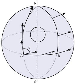
In differential geometry, parallel transport (or parallel translation^a) is a way of transporting geometrical data along smooth curves in a manifold. If the manifold is equipped with an affine connection (a covariant derivative or connection on the tangent bundle), then this connection allows one to transport vectors of the manifold along curves so that they stay parallel with respect to the connection.

The parallel transport for a connection thus supplies a way of, in some sense, moving the local geometry of a manifold along a curve: that is, of connecting the geometries of nearby points. There may be many notions of parallel transport available, but a specification of one way of connecting up the geometries of points on a curve is tantamount to providing a connection. In fact, the usual notion of connection is the infinitesimal analog of parallel transport. Or, vice versa, parallel transport is the local realization of a connection.

As parallel transport supplies a local realization of the connection, it also supplies a local realization of the curvature known as holonomy. The Ambrose–Singer theorem makes explicit this relationship between the curvature and holonomy.

Other notions of connection come equipped with their own parallel transportation systems as well. For instance, a Koszul connection in a vector bundle also allows for the parallel transport of vectors in much the same way as with a covariant derivative. An Ehresmann or Cartan connection supplies a lifting of curves from the manifold to the total space of a principal bundle. Such curve lifting may sometimes be thought of as the parallel transport of reference frames.

In Euclidean geometry, straight lines, on the one hand, minimize arc length among all curves connecting two given points. On the other hand, their direction remains constant along them; equivalently, their tangent vectors are parallel transported along them.

In the theory of differentiable manifolds, additional structure is required to make sense of arc length and parallel transport. The former is provided by a Riemannian structure, leading to the notion of a metric geodesic, while the latter is provided by a connection, leading to the notions of parallel transport and affine geodesics.

Let us consider the sphere, ${\displaystyle S^{2}}$, as an example of a smooth manifold. If we regard it as a subset of its ambient 3-dimensional Euclidean space, then it makes sense to speak about vectors tangent to ${\displaystyle S^{2}}$ at a point ${\displaystyle p\in S^{2}}$. All tangent vectors at this point form a 2-dimensional subspace of the ambient vector space, and we can call this 2-dimensional vector space the tangent space of ${\displaystyle S^{2}}$ at ${\displaystyle p}$. In the theory of smooth manifolds, ${\displaystyle S^{2}}$ is regarded in its own right, without any ambient space, and a tangent space at ${\displaystyle p}$ is defined internally, as the vector space of derivations at ${\displaystyle p}$. The tangent space at ${\displaystyle p\in S^{2}}$ is denoted by ${\displaystyle T_{p}S^{2}}$, and for a general differentiable manifold ${\displaystyle M}$ by ${\displaystyle T_{p}M}$. The concept of parallel transport was introduced to address the fact that there is no canonical identification between tangent vectors at different points of a manifold. In general, this problem cannot be solved globally, but only along differentiable curves in the manifold.

In our example, in analogy with straight lines in Euclidean space, we may say that the tangent vector field along a geodesic in a Riemannian manifold (the analogue of a straight line in Euclidean space) “does not change”; that is, the tangent vectors are parallel transports of one another along the geodesic. Likewise, unit vectors orthogonal to the tangent vectors are also parallel transported along the geodesic. By linearity, this determines the parallel transport of any tangent vector along the geodesic.

Generally, the parallel transport of tangent vectors along a curve requires additional structure beyond the smooth structure. In our example above, we supposed the existence of a Riemannian metric on the sphere, which determines the geodesics (the curves with extremal length), and the rule of parallel transport is supposed to be in accordance with this Riemannian structure. But the concept of parallel transport is more general. The rule, how the tangent vectors of the manifold should transport parallelly along a curve, can be itself this "additional structure", since it can be defined even if the manifold doesn't have any additional structure beyond the smooth structure. It can be done as follows. All tangent vectors at every point of a manifold ${\displaystyle M}$ form the tangent bundle ${\displaystyle TM}$ of ${\displaystyle M}$. Taking a curve ${\displaystyle c:I\subseteq \mathbb {R} \to M}$, and picking a tangent vector ${\displaystyle v(c(t))\in T_{p}M}$ at each point ${\displaystyle c(t)}$, the resulting function ${\displaystyle v:I\to TM:t\mapsto v(c(t))}$ is a curve in ${\displaystyle TM}$. The general rule of parallel transport specifies when the tangent vector of ${\displaystyle v}$ should be regarded "horizontal". If the tangent vectors of ${\displaystyle v}$ (which are in ${\displaystyle TTM}$) are horizontal at each point, we say that ${\displaystyle v}$ is a horizontal curve in ${\displaystyle TM}$, or that ${\displaystyle v}$ is parallelly transported along ${\displaystyle c}$. The rule that specifies whether a tangent vector of the curve ${\displaystyle v}$ is horizontal or not, called a connection. It specifies the horizontal subspaces in ${\displaystyle T_{y}TM}$ for each ${\displaystyle y\in TM}$, and thus defines parallel transport.

Let ${\displaystyle M}$ be a smooth manifold. For each point ⁠${\displaystyle p\in M}$⁠, there is an associated vector space ${\displaystyle T_{p}M}$ called the tangent space of ${\displaystyle M}$ at ${\displaystyle p}$. Vectors in ${\displaystyle T_{p}M}$ are thought of as the vectors tangent to ${\displaystyle M}$ at ${\displaystyle p}$. A Riemannian metric ${\displaystyle g}$ on ${\displaystyle M}$ assigns to each ${\displaystyle p}$ a positive-definite inner product ${\displaystyle g_{p}:T_{p}M\times T_{p}M\to \mathbf {R} }$ in a smooth way. A smooth manifold ${\displaystyle M}$ endowed with a Riemannian metric ${\displaystyle g}$ is a Riemannian manifold, denoted ⁠${\displaystyle (M,g)}$⁠.

Let ${\displaystyle x^{1},\ldots ,x^{n}}$ denote the standard coordinates on ${\displaystyle \mathbf {R} ^{n}.}$ The Euclidean metric ${\displaystyle g^{\text{euc}}}$ is given by

${\displaystyle g^{\text{euc}}=(dx^{1})^{2}+\cdots +(dx^{n})^{2}}$.²

Euclidean space is the Riemannian manifold ${\displaystyle (\mathbf {R} ^{n},g^{\text{euc}})}$.

In Euclidean space, all tangent spaces are canonically identified with each other via translation, so it is easy to move vectors from one tangent space to another. Parallel transport of tangent vectors is a way of moving vectors from one tangent space to another along a curve in the setting of a general Riemannian manifold. Note that while the vectors are in the tangent space of the manifold, they might not be in the tangent space of the curve they are being transported along.

An affine connection on a Riemannian manifold is a way of differentiating vector fields with respect to other vector fields. A Riemannian manifold has a natural choice of affine connection called the Levi-Civita connection. Given a fixed affine connection on a Riemannian manifold, there is a unique way to do parallel transport of tangent vectors.³ Different choices of affine connections will lead to different systems of parallel transport.

Let ${\displaystyle M}$ be a manifold with an affine connection ⁠${\displaystyle \nabla }$⁠. Then a vector field ${\displaystyle X}$ is said to be parallel if for any vector field ⁠${\displaystyle Y}$⁠, ⁠${\displaystyle \nabla _{Y}X=0}$⁠. Intuitively speaking, parallel vector fields have all their derivatives equal to zero and are therefore in some sense constant. By evaluating a parallel vector field at two points ${\displaystyle x}$ and ⁠${\displaystyle y}$⁠, an identification between a tangent vector at ${\displaystyle x}$ and one at ${\displaystyle y}$ is obtained. Such tangent vectors are said to be parallel transports of each other.

More precisely, if ${\displaystyle \gamma :I\rightarrow M}$ is a piecewise continuously differentiable curve parametrized by an interval ${\displaystyle [a,b]}$ and ⁠${\displaystyle \xi \in T_{x}M}$⁠, where ⁠${\displaystyle x=\gamma (a)}$⁠, then a vector field ${\displaystyle X}$ along ${\displaystyle \gamma }$ (and in particular, the value of this vector field at ⁠${\displaystyle y=\gamma (b)}$⁠) is called the parallel transport of ${\displaystyle \xi }$ along ${\displaystyle \gamma }$ if

1. ${\displaystyle \nabla _{\gamma '(t)}X=0,{\text{ for all }}t\in [a,b]}$
2. ${\displaystyle X_{\gamma (a)}=\xi .}$

Formally, the first condition means that ${\displaystyle X}$ is parallel with respect to the pullback connection on the pullback bundle ⁠${\displaystyle \gamma ^{*}TM}$⁠. However, in a local trivialization it is a first-order system of linear ordinary differential equations, which has a unique solution for any initial condition given by the second condition (for instance, by the Picard–Lindelöf theorem).

The parallel transport of ${\displaystyle X\in T_{\gamma (s)}M}$ to the tangent space ${\displaystyle T_{\gamma (t)}M}$ along the curve ${\displaystyle \gamma :[0,1]\to M}$ is denoted by ⁠${\displaystyle \Gamma (\gamma )_{s}^{t}X}$⁠. The map

${\displaystyle \Gamma (\gamma )_{s}^{t}:T_{\gamma (s)}M\to T_{\gamma (t)}M}$

is linear. In fact, it is an isomorphism. Let ${\displaystyle {\overline {\gamma }}:[0,1]\to M}$ be the inverse curve ${\displaystyle {\overline {\gamma }}(t)=\gamma (1-t).}$ Then ${\displaystyle \Gamma ({\overline {\gamma }})_{t}^{s}}$ is the inverse of ⁠${\displaystyle \Gamma (\gamma )_{s}^{t}}$⁠.

To summarize, parallel transport provides a way of moving tangent vectors along a curve using the affine connection to keep them "pointing in the same direction" in an intuitive sense, and this provides a linear isomorphism between the tangent spaces at the two ends of the curve. The isomorphism obtained in this way will in general depend on the choice of the curve. If it does not, then parallel transport along every curve can be used to define parallel vector fields on M, which can only happen if the curvature of ∇ is zero.

A linear isomorphism is determined by its action on an ordered basis or frame. Hence parallel transport can also be characterized as a way of transporting elements of the (tangent) frame bundle GL(M) along a curve. In other words, the affine connection provides a lift of any curve γ in M to a curve γ̃ in GL(M).

The images below show parallel transport induced by the Levi-Civita connection associated to two different Riemannian metrics on the punctured plane ⁠${\displaystyle \mathbf {R} ^{2}\smallsetminus \{0,0\}}$⁠. The curve the parallel transport is done along is the unit circle. In polar coordinates, the metric on the left is the standard Euclidean metric ⁠${\displaystyle dx^{2}+dy^{2}=dr^{2}+r^{2}\,d\theta ^{2}}$⁠, while the metric on the right is ⁠${\displaystyle dr^{2}+d\theta ^{2}}$⁠. This second metric has a singularity at the origin, so it does not extend past the puncture, but the first metric extends to the entire plane.

Parallel transports on the punctured plane under Levi-Civita connections

This transport is given by the metric ⁠${\displaystyle dr^{2}+r^{2}\,d\theta ^{2}}$⁠.

This transport is given by the metric ⁠${\displaystyle dr^{2}+d\theta ^{2}}$⁠.

Warning: This is parallel transport on the punctured plane along the unit circle, not parallel transport on the unit circle. Indeed, in the first image, the vectors fall outside of the tangent space to the unit circle. Since the first metric has zero curvature, the transport between two points along the circle could be accomplished along any other curve as well. However, the second metric has non-zero curvature, and the circle is a geodesic, so that its field of tangent vectors is parallel.

A metric connection is any connection whose parallel transport mappings preserve the Riemannian metric, that is, for any curve ${\displaystyle \gamma }$ and any two vectors ⁠${\displaystyle X,Y\in T_{\gamma (s)}M}$⁠,

${\displaystyle \langle \Gamma (\gamma )_{s}^{t}X,\Gamma (\gamma )_{s}^{t}Y\rangle _{\gamma (t)}=\langle X,Y\rangle _{\gamma (s)}.}$

Taking the derivative at t = 0, the operator ∇ satisfies a product rule with respect to the metric, namely

${\displaystyle Z\langle X,Y\rangle =\langle \nabla _{Z}X,Y\rangle +\langle X,\nabla _{Z}Y\rangle .}$

An affine connection distinguishes a class of curves called (affine) geodesics.⁴ A curve ${\displaystyle \gamma :I\rightarrow M}$ is an affine geodesic if ${\displaystyle {\dot {\gamma }}}$ is parallel transported along ⁠${\displaystyle \gamma }$⁠, that is

${\displaystyle \Gamma (\gamma )_{s}^{t}{\dot {\gamma }}(s)={\dot {\gamma }}(t).}$

Taking the derivative with respect to time, this takes the more familiar form

${\displaystyle \nabla _{{\dot {\gamma }}(t)}{\dot {\gamma }}=0.}$

If ${\displaystyle \nabla }$ is a metric connection, then the affine geodesics are the usual geodesics of Riemannian geometry and are the locally distance minimizing curves. More precisely, first note that if ${\displaystyle \gamma :I\rightarrow M}$, where ${\displaystyle I}$ is an open interval, is a geodesic, then the norm of ${\displaystyle {\dot {\gamma }}}$ is constant on ⁠${\displaystyle I}$⁠. Indeed,

${\displaystyle {\frac {d}{dt}}\langle {\dot {\gamma }}(t),{\dot {\gamma }}(t)\rangle =2\langle \nabla _{{\dot {\gamma }}(t)}{\dot {\gamma }}(t),{\dot {\gamma }}(t)\rangle =0.}$

It follows from an application of Gauss's lemma that if ${\displaystyle A}$ is the norm of ${\displaystyle {\dot {\gamma }}(t)}$ then the distance, induced by the metric, between two close enough points on the curve ⁠${\displaystyle \gamma }$⁠, say ${\displaystyle \gamma (t_{1})}$ and ⁠${\displaystyle \gamma (t_{2})}$⁠, is given by $${\displaystyle {\mbox{dist}}{\big (}\gamma (t_{1}),\gamma (t_{2}){\big )}=A|t_{1}-t_{2}|.}$$ The formula above might not be true for points which are not close enough since the geodesic might for example wrap around the manifold (e.g. on a sphere).

Parallel transport of tangent vectors is a special case of a more general construction involving an arbitrary vector bundle ${\displaystyle E}$. Specifically, parallel transport of tangent vectors is the case where ${\displaystyle E}$ is the tangent bundle ${\displaystyle TM}$.

Let M be a smooth manifold. Let E → M be a vector bundle with connection ∇ and γ: I → M a curve parameterized by an open interval I. A section ${\displaystyle X}$ of ${\displaystyle E}$ along γ is called parallel if

${\displaystyle \nabla _{{\dot {\gamma }}(t)}X=0{\text{ for }}t\in I.}$

In the case when ${\displaystyle E}$ is the tangent bundle whereby ${\displaystyle X}$ is a tangent vector field, this expression means that, for every ${\displaystyle t}$ in the interval, tangent vectors in ${\displaystyle X}$ are "constant" (the derivative vanishes) when an infinitesimal displacement from ${\displaystyle \gamma (t)}$ in the direction of the tangent vector ${\displaystyle {\dot {\gamma }}(t)}$ is done.

Suppose we are given an element e₀ ∈ E_P at P = γ(0) ∈ M, rather than a section. The parallel transport of e₀ along γ is the extension of e₀ to a parallel section X on γ. More precisely, X is the unique part of E along γ such that

1. ${\displaystyle \nabla _{\dot {\gamma }}X=0}$
2. ${\displaystyle X_{\gamma (0)}=e_{0}.}$

Note that in any given coordinate patch, (1) defines an ordinary differential equation, with the initial condition given by (2). Thus the Picard–Lindelöf theorem guarantees the existence and uniqueness of the solution.

Thus the connection ∇ defines a way of moving elements of the fibers along a curve, and this provides linear isomorphisms between the fibers at points along the curve:

${\displaystyle \Gamma (\gamma )_{s}^{t}:E_{\gamma (s)}\rightarrow E_{\gamma (t)}}$

from the vector space lying over γ(s) to that over γ(t). This isomorphism is known as the parallel transport map associated to the curve. The isomorphisms between fibers obtained in this way will, in general, depend on the choice of the curve: if they do not, then parallel transport along every curve can be used to define parallel sections of E over all of M. This is only possible if the curvature of ∇ is zero.

In particular, parallel transport around a closed curve starting at a point x defines an automorphism of the tangent space at x which is not necessarily trivial. The parallel transport automorphisms defined by all closed curves based at x form a transformation group called the holonomy group of ∇ at x. There is a close relation between this group and the value of the curvature of ∇ at x; this is the content of the Ambrose–Singer holonomy theorem.

Given a covariant derivative ∇, the parallel transport along a curve γ is obtained by integrating the condition ⁠${\displaystyle \textstyle {\nabla _{\dot {\gamma }}=0}}$⁠. Conversely, if a suitable notion of parallel transport is available, then a corresponding connection can be obtained by differentiation. This approach is due, essentially, to Knebelman (1951); see Guggenheimer (1977). Lumiste (2001) also adopts this approach.

Consider an assignment to each curve γ in the manifold a collection of mappings

${\displaystyle \Gamma (\gamma )_{s}^{t}:E_{\gamma (s)}\rightarrow E_{\gamma (t)}}$

such that

1. ${\displaystyle \Gamma (\gamma )_{s}^{s}=Id}$, the identity transformation of E_γ(s).
2. ${\displaystyle \Gamma (\gamma )_{u}^{t}\circ \Gamma (\gamma )_{s}^{u}=\Gamma (\gamma )_{s}^{t}.}$
3. The dependence of Γ on γ, s, and t is "smooth".

The notion of smoothness in condition 3. is somewhat difficult to pin down (see the discussion below of parallel transport in fibre bundles). In particular, modern authors such as Kobayashi and Nomizu generally view the parallel transport of the connection as coming from a connection in some other sense, where smoothness is more easily expressed.

Nevertheless, given such a rule for parallel transport, it is possible to recover the associated infinitesimal connection in E as follows. Let γ be a differentiable curve in M with initial point γ(0) and initial tangent vector X = γ′(0). If V is a section of E over γ, then let

${\displaystyle \nabla _{X}V=\lim _{h\to 0}{\frac {\Gamma (\gamma )_{h}^{0}V_{\gamma (h)}-V_{\gamma (0)}}{h}}=\left.{\frac {d}{dt}}\Gamma (\gamma )_{t}^{0}V_{\gamma (t)}\right|_{t=0}.}$

This defines the associated infinitesimal connection ∇ on E. One recovers the same parallel transport Γ from this infinitesimal connection.

The parallel transport can be defined in greater generality for other types of connections, not just those defined in a vector bundle. One generalization is for principal connections (Kobayashi & Nomizu 1996, Volume 1, Chapter II). Let P → M be a principal bundle over a manifold M with structure Lie group G and a principal connection ω. As in the case of vector bundles, a principal connection ω on P defines, for each curve γ in M, a mapping

${\displaystyle \Gamma (\gamma )_{s}^{t}:P_{\gamma (s)}\rightarrow P_{\gamma (t)}}$

from the fibre over γ(s) to that over γ(t), which is an isomorphism of homogeneous spaces: i.e. ${\displaystyle \Gamma _{\gamma (s)}g=g\Gamma _{\gamma (s)}}$ for each g ∈ G.

Further generalizations of parallel transport are also possible. In the context of Ehresmann connections, where the connection depends on a special notion of "horizontal lifting" of tangent spaces, one can define parallel transport via horizontal lifts. Cartan connections are Ehresmann connections with additional structure which allows the parallel transport to be thought of as a map "rolling" a certain model space along a curve in the manifold. This rolling is called development.

Parallel transport can be discretely approximated by Schild's ladder, which takes finite steps along a curve, and approximates Levi-Civita parallelogramoids by approximate parallelograms.

References

- Guggenheimer, Heinrich (1977), Differential Geometry, Dover, ISBN 0-486-63433-7
- Knebelman (1951), "Spaces of relative parallelism", Annals of Mathematics, 2, 53 (3), The Annals of Mathematics, Vol. 53, No. 3: 387–399, doi:10.2307/1969562, JSTOR 1969562
- Kobayashi, Shoshichi; Nomizu, Katsumi (1996), Foundations of Differential Geometry, Volume 1, Wiley-Interscience, ISBN 0-471-15733-3; Volume 2, ISBN 0-471-15732-5.
- Lumiste, Ü. (2001) [1994], "Connections on a manifold", Encyclopedia of Mathematics, EMS Press
- Spivak, Michael (1999). A Comprehensive Introduction to Differential Geometry, Vol. II. Publish-or-Perish Press. ISBN 0914098713.
- Lee, John M. (2018). Introduction to Riemannian Manifolds. Springer-Verlag. ISBN 978-3-319-91754-2.
External links
- Spherical Geometry Demo Archived 2007-05-19 at the Wayback Machine. An applet demonstrating parallel transport of tangent vectors on a sphere.