Multipole magnet

Multipole magnets are magnets built from multiple individual magnets, typically used to control beams of charged particles. Each type of magnet serves a particular purpose.

• Dipole magnets are used to bend the trajectory of particles
• Quadrupole magnets are used to focus particle beams
• Sextupole magnets are used to correct for chromaticity introduced by quadrupole magnets¹

The magnetic field of an ideal multipole magnet in an accelerator is typically modeled as having no (or a constant) component parallel to the nominal beam direction (${\displaystyle z}$ direction) and the transverse components can be written as complex numbers:²

${\displaystyle B_{y}+iB_{x}=C_{n}\cdot (x-iy)^{n-1}}$

where ${\displaystyle x}$ and ${\displaystyle y}$ are the coordinates in the plane transverse to the nominal beam direction. ${\displaystyle C_{n}}$ is a complex number specifying the orientation and strength of the magnetic field. ${\displaystyle B_{x}}$ and ${\displaystyle B_{y}}$ are the components of the magnetic field in the corresponding directions. Fields with a real ${\displaystyle C_{n}}$ are called 'normal' while fields with ${\displaystyle C_{n}}$ purely imaginary are called 'skewed'.

First few multipole fields

n	name	magnetic field lines	example device
1	dipole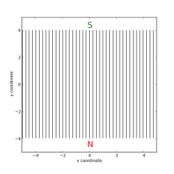
2	quadrupole
3	sextupole

For an electromagnet with a cylindrical bore, producing a pure multipole field of order ${\displaystyle n}$, the stored magnetic energy is:

${\displaystyle U_{n}={\frac {n!^{2}}{2n}}\pi \mu _{0}\ell N^{2}I^{2}.}$

Here, ${\displaystyle \mu _{0}}$ is the permeability of free space, ${\displaystyle \ell }$ is the effective length of the magnet (the length of the magnet, including the fringing fields), ${\displaystyle N}$ is the number of turns in one of the coils (such that the entire device has ${\displaystyle 2nN}$ turns), and ${\displaystyle I}$ is the current flowing in the coils. Formulating the energy in terms of ${\displaystyle NI}$ can be useful, since the magnitude of the field and the bore radius do not need to be measured.

Note that for a non-electromagnet, this equation still holds if the magnetic excitation can be expressed in Amperes.

The equation for stored energy in an arbitrary magnetic field is:³

${\displaystyle U={\frac {1}{2}}\int \left({\frac {B^{2}}{\mu _{0}}}\right)\,d\tau .}$

Here, ${\displaystyle \mu _{0}}$ is the permeability of free space, ${\displaystyle B}$ is the magnitude of the field, and ${\displaystyle d\tau }$ is an infinitesimal element of volume. Now for an electromagnet with a cylindrical bore of radius ${\displaystyle R}$, producing a pure multipole field of order ${\displaystyle n}$, this integral becomes:

${\displaystyle U_{n}={\frac {1}{2\mu _{0}}}\int ^{\ell }\int _{0}^{R}\int _{0}^{2\pi }B^{2}\,d\tau .}$

Ampere's Law for multipole electromagnets gives the field within the bore as:⁴

${\displaystyle B(r)={\frac {n!\mu _{0}NI}{R^{n}}}r^{n-1}.}$

Here, ${\displaystyle r}$ is the radial coordinate. It can be seen that along ${\displaystyle r}$ the field of a dipole is constant, the field of a quadrupole magnet is linearly increasing (i.e. has a constant gradient), and the field of a sextupole magnet is parabolically increasing (i.e. has a constant second derivative). Substituting this equation into the previous equation for ${\displaystyle U_{n}}$ gives:

${\displaystyle U_{n}={\frac {1}{2\mu _{0}}}\int ^{\ell }\int _{0}^{R}\int _{0}^{2\pi }\left({\frac {n!\mu _{0}NI}{R^{n}}}r^{n-1}\right)^{2}\,d\tau ,}$

${\displaystyle U_{n}={\frac {1}{2\mu _{0}}}\int _{0}^{R}\left({\frac {n!\mu _{0}NI}{R^{n}}}r^{n-1}\right)^{2}(2\pi \ell r\,dr),}$

${\displaystyle U_{n}={\frac {\pi \mu _{0}\ell n!^{2}N^{2}I^{2}}{R^{2n}}}\int _{0}^{R}r^{2n-1}\,dr,}$

${\displaystyle U_{n}={\frac {\pi \mu _{0}\ell n!^{2}N^{2}I^{2}}{R^{2n}}}\left({\frac {R^{2n}}{2n}}\right),}$

${\displaystyle U_{n}={\frac {n!^{2}}{2n}}\pi \mu _{0}\ell N^{2}I^{2}.}$

References

- "Varna 2010 | the CERN Accelerator School" (PDF). Archived from the original (PDF) on 2017-05-13.
- "Wolski, Maxwell's Equations for Magnets – CERN Accelerator School 2009".
- Griffiths, David (2013). Introduction to Electromagnetism (4th ed.). Illinois: Pearson. p. 329.
- Tanabe, Jack (2005). Iron Dominated Electromagnets - Design, Fabrication, Assembly and Measurements (4th ed.). Singapore: World Scientific.