Logarithmic distribution

Logarithmic
Probability mass function 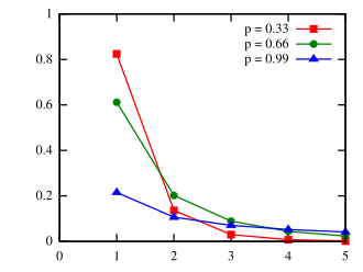The function is only defined at integer values. The connecting lines are merely guides for the eye.
Cumulative distribution function
Parameters	${\displaystyle 0<p<1}$
Support	${\displaystyle k\in \{1,2,3,\ldots \}}$
PMF	${\displaystyle {\frac {-1}{\ln(1-p)}}{\frac {p^{k}}{k}}}$
CDF	${\displaystyle 1+{\frac {\mathrm {B} (p;k+1,0)}{\ln(1-p)}}}$
Mean	${\displaystyle {\frac {-1}{\ln(1-p)}}{\frac {p}{1-p}}}$
Mode	${\displaystyle 1}$
Variance	${\displaystyle -{\frac {p^{2}+p\ln(1-p)}{(1-p)^{2}(\ln(1-p))^{2}}}}$
MGF	${\displaystyle {\frac {\ln(1-pe^{t})}{\ln(1-p)}}{\text{ for }}t<-\ln p}$
CF	${\displaystyle {\frac {\ln(1-pe^{it})}{\ln(1-p)}}}$
PGF	${\displaystyle {\frac {\ln(1-pz)}{\ln(1-p)}}{\text{ for }}|z|<{\frac {1}{p}}}$

In probability and statistics, the logarithmic distribution (also known as the logarithmic series distribution or the log-series distribution) is a discrete probability distribution derived from the Maclaurin series expansion

${\displaystyle -\ln(1-p)=p+{\frac {p^{2}}{2}}+{\frac {p^{3}}{3}}+\cdots .}$

From this we obtain the identity

${\displaystyle \sum _{k=1}^{\infty }{\frac {-1}{\ln(1-p)}}\;{\frac {p^{k}}{k}}=1.}$

This leads directly to the probability mass function of a Log(p)-distributed random variable:

${\displaystyle f(k)={\frac {-1}{\ln(1-p)}}\;{\frac {p^{k}}{k}}}$

for k ≥ 1, and where 0 < p < 1. Because of the identity above, the distribution is properly normalized.

The cumulative distribution function is

${\displaystyle F(k)=1+{\frac {\mathrm {B} (p;k+1,0)}{\ln(1-p)}}}$

where B is the incomplete beta function.

A Poisson compounded with Log(p)-distributed random variables has a negative binomial distribution. In other words, if N is a random variable with a Poisson distribution, and X_i, i = 1, 2, 3, ... is an infinite sequence of independent identically distributed random variables each having a Log(p) distribution, then

${\displaystyle \sum _{i=1}^{N}X_{i}}$

has a negative binomial distribution. In this way, the negative binomial distribution is seen to be a compound Poisson distribution.

R. A. Fisher described the logarithmic distribution in a paper that used it to model relative species abundance.¹

References

- Fisher, R. A.; Corbet, A. S.; Williams, C. B. (1943). "The Relation Between the Number of Species and the Number of Individuals in a Random Sample of an Animal Population" (PDF). Journal of Animal Ecology. 12 (1): 42–58. Bibcode:1943JAnEc..12...42F. doi:10.2307/1411. JSTOR 1411. Archived from the original (PDF) on 2011-07-26.
Further reading
- Johnson, Norman Lloyd; Kemp, Adrienne W.; Kotz, Samuel (2005). "Chapter 7: Logarithmic and Lagrangian distributions". Univariate discrete distributions (3 ed.). John Wiley & Sons. ISBN 978-0-471-27246-5.
- Weisstein, Eric W. "Log-Series Distribution". MathWorld.