Article · Wikipedia archive · Last revised Jun 21, 2026

Liouville function

In number theory, the Liouville function, named after French mathematician Joseph Liouville and denoted , is an important arithmetic function. Its value is if is the product of an even number of prime numbers, and if it is the product of an odd number of prime numbers.

Last revised
Jun 21, 2026
Read time
≈ 9 min
Length
2,098 w
Citations
5
Source

In number theory, the Liouville function, named after French mathematician Joseph Liouville and denoted λ ( n ) {\displaystyle \lambda (n)} , is an important arithmetic function. Its value is 1 {\displaystyle 1} if n {\displaystyle n} is the product of an even number of prime numbers, and 1 {\displaystyle -1} if it is the product of an odd number of prime numbers.

Definition

By the fundamental theorem of arithmetic, any positive integer n {\displaystyle n} can be represented uniquely as a product of powers of primes:

n = p 1 a 1 p k a k {\displaystyle n=p_{1}^{a_{1}}\cdots p_{k}^{a_{k}}} ,

where p 1 , , p k {\displaystyle p_{1},\dots ,p_{k}} are primes and the exponents a 1 , , a k {\displaystyle a_{1},\dots ,a_{k}} are positive integers. The prime omega function Ω ( n ) {\displaystyle \Omega (n)} counts the number of primes in the factorization of n {\displaystyle n} with multiplicity:

Ω ( n ) = a 1 + a 2 + + a k {\displaystyle \Omega (n)=a_{1}+a_{2}+\cdots +a_{k}} .

Thus, the Liouville function is defined by

λ ( n ) = ( 1 ) Ω ( n ) {\displaystyle \lambda (n)=(-1)^{\Omega (n)}}

(sequence A008836 in the OEIS).

Properties

Since Ω ( n ) {\displaystyle \Omega (n)} is completely additive; i.e., Ω ( a b ) = Ω ( a ) + Ω ( b ) {\displaystyle \Omega (ab)=\Omega (a)+\Omega (b)} , then λ ( n ) {\displaystyle \lambda (n)} is completely multiplicative. Since 1 {\displaystyle 1} has no prime factors, Ω ( 1 ) = 0 {\displaystyle \Omega (1)=0} , so λ ( 1 ) = 1 {\displaystyle \lambda (1)=1} .

λ ( n ) {\displaystyle \lambda (n)} is also related to the Möbius function μ ( n ) {\displaystyle \mu (n)} : if we write n {\displaystyle n} as n = a 2 b {\displaystyle n=a^{2}b} , where b {\displaystyle b} is squarefree, then

λ ( n ) = μ ( b ) . {\displaystyle \lambda (n)=\mu (b).}

The sum of the Liouville function over the divisors of n {\displaystyle n} is the characteristic function of the squares:

d | n λ ( d ) = { 1 if  n  is a perfect square, 0 otherwise. {\displaystyle \sum _{d|n}\lambda (d)={\begin{cases}1&{\text{if }}n{\text{ is a perfect square,}}\\0&{\text{otherwise.}}\end{cases}}}

Möbius inversion of this formula yields

λ ( n ) = d 2 | n μ ( n d 2 ) . {\displaystyle \lambda (n)=\sum _{d^{2}|n}\mu \left({\frac {n}{d^{2}}}\right).}

The Dirichlet inverse of the Liouville function is the absolute value of the Möbius function, λ 1 ( n ) = | μ ( n ) | = μ 2 ( n ) {\displaystyle \lambda ^{-1}(n)=|\mu (n)|=\mu ^{2}(n)} , the characteristic function of the squarefree integers.

Series

The Dirichlet series for the Liouville function is related to the Riemann zeta function by

ζ ( 2 s ) ζ ( s ) = n = 1 λ ( n ) n s . {\displaystyle {\frac {\zeta (2s)}{\zeta (s)}}=\sum _{n=1}^{\infty }{\frac {\lambda (n)}{n^{s}}}.}

Also:

n = 1 λ ( n ) ln n n = ζ ( 2 ) = π 2 6 . {\displaystyle \sum \limits _{n=1}^{\infty }{\frac {\lambda (n)\ln n}{n}}=-\zeta (2)=-{\frac {\pi ^{2}}{6}}.}

The Lambert series for the Liouville function is

n = 1 λ ( n ) q n 1 q n = n = 1 q n 2 = 1 2 ( ϑ 3 ( q ) 1 ) , {\displaystyle \sum _{n=1}^{\infty }{\frac {\lambda (n)q^{n}}{1-q^{n}}}=\sum _{n=1}^{\infty }q^{n^{2}}={\frac {1}{2}}\left(\vartheta _{3}(q)-1\right),}

where ϑ 3 ( q ) {\displaystyle \vartheta _{3}(q)} is the Jacobi theta function.

Conjectures on weighted summatory functions

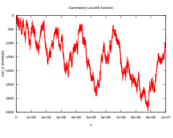
Summatory Liouville function L(n) up to n = 104. The readily visible oscillations are due to the first non-trivial zero of the Riemann zeta function. source ↗
Summatory Liouville function L(n) up to n = 107. Note the apparent scale invariance of the oscillations. source ↗
Logarithmic graph of the negative of the summatory Liouville function L(n) up to n = 2 × 109. The green spike shows the function itself (not its negative) in the narrow region where the Pólya conjecture fails; the blue curve shows the oscillatory contribution of the first Riemann zero. source ↗
Harmonic Summatory Liouville function T(n) up to n = 103 source ↗

The Pólya problem is a question raised made by George Pólya in 1919. Defining

L ( n ) = k = 1 n λ ( k ) {\displaystyle L(n)=\sum _{k=1}^{n}\lambda (k)} (sequence A002819 in the OEIS),

the problem asks whether L(n) ≤ 0 for all n > 1. The answer turns out to be no. The smallest counter-example is n = 906150257, found by Minoru Tanaka in 1980. It has since been shown that L(n) > 0.0618672n for infinitely many positive integers n,1 while it can also be shown via the same methods that L(n) < −1.3892783n for infinitely many positive integers n.2

For any ε > 0 {\displaystyle \varepsilon >0} , assuming the Riemann hypothesis, we have that the summatory function L ( x ) L 0 ( x ) {\displaystyle L(x)\equiv L_{0}(x)} is bounded by

L ( x ) = O ( x exp ( C log 1 / 2 ( x ) ( log log x ) 5 / 2 + ε ) ) , {\displaystyle L(x)=O\left({\sqrt {x}}\exp \left(C\cdot \log ^{1/2}(x)\left(\log \log x\right)^{5/2+\varepsilon }\right)\right),}

where the C > 0 {\displaystyle C>0} is some absolute limiting constant.2

Define the related sum

T ( n ) = k = 1 n λ ( k ) k . {\displaystyle T(n)=\sum _{k=1}^{n}{\frac {\lambda (k)}{k}}.}

It was open for some time whether T(n) ≥ 0 for sufficiently big nn0 (this conjecture is occasionally—though incorrectly—attributed to Pál Turán). This was then disproved by Haselgrove (1958), who showed that T(n) takes negative values infinitely often. A confirmation of this positivity conjecture would have led to a proof of the Riemann hypothesis, as was shown by Pál Turán.

Generalizations

More generally, we can consider the weighted summatory functions over the Liouville function defined for any α R {\displaystyle \alpha \in \mathbb {R} } as follows for positive integers x where (as above) we have the special cases L ( x ) := L 0 ( x ) {\displaystyle L(x):=L_{0}(x)} and T ( x ) = L 1 ( x ) {\displaystyle T(x)=L_{1}(x)} 2

L α ( x ) := n x λ ( n ) n α . {\displaystyle L_{\alpha }(x):=\sum _{n\leq x}{\frac {\lambda (n)}{n^{\alpha }}}.}

These α 1 {\displaystyle \alpha ^{-1}} -weighted summatory functions are related to the Mertens function, or weighted summatory functions of the Möbius function. In fact, we have that the so-termed non-weighted, or ordinary, function L ( x ) {\displaystyle L(x)} precisely corresponds to the sum

L ( x ) = d 2 x M ( x d 2 ) = d 2 x n x d 2 μ ( n ) . {\displaystyle L(x)=\sum _{d^{2}\leq x}M\left({\frac {x}{d^{2}}}\right)=\sum _{d^{2}\leq x}\sum _{n\leq {\frac {x}{d^{2}}}}\mu (n).}

Moreover, these functions satisfy similar bounding asymptotic relations.2 For example, whenever 0 α 1 2 {\displaystyle 0\leq \alpha \leq {\frac {1}{2}}} , we see that there exists an absolute constant C α > 0 {\displaystyle C_{\alpha }>0} such that

L α ( x ) = O ( x 1 α exp ( C α ( log x ) 3 / 5 ( log log x ) 1 / 5 ) ) . {\displaystyle L_{\alpha }(x)=O\left(x^{1-\alpha }\exp \left(-C_{\alpha }{\frac {(\log x)^{3/5}}{(\log \log x)^{1/5}}}\right)\right).}

By an application of Perron's formula, or equivalently by a key (inverse) Mellin transform, we have that

ζ ( 2 α + 2 s ) ζ ( α + s ) = s 1 L α ( x ) x s + 1 d x , {\displaystyle {\frac {\zeta (2\alpha +2s)}{\zeta (\alpha +s)}}=s\cdot \int _{1}^{\infty }{\frac {L_{\alpha }(x)}{x^{s+1}}}dx,}

which then can be inverted via the inverse transform to show that for x > 1 {\displaystyle x>1} , T 1 {\displaystyle T\geq 1} and 0 α < 1 2 {\displaystyle 0\leq \alpha <{\frac {1}{2}}}

L α ( x ) = 1 2 π ı σ 0 ı T σ 0 + ı T ζ ( 2 α + 2 s ) ζ ( α + s ) x s s d s + E α ( x ) + R α ( x , T ) , {\displaystyle L_{\alpha }(x)={\frac {1}{2\pi \imath }}\int _{\sigma _{0}-\imath T}^{\sigma _{0}+\imath T}{\frac {\zeta (2\alpha +2s)}{\zeta (\alpha +s)}}\cdot {\frac {x^{s}}{s}}ds+E_{\alpha }(x)+R_{\alpha }(x,T),}

where we can take σ 0 := 1 α + 1 / log ( x ) {\displaystyle \sigma _{0}:=1-\alpha +1/\log(x)} , and with the remainder terms defined such that E α ( x ) = O ( x α ) {\displaystyle E_{\alpha }(x)=O(x^{-\alpha })} and R α ( x , T ) 0 {\displaystyle R_{\alpha }(x,T)\rightarrow 0} as T {\displaystyle T\rightarrow \infty } .

In particular, if we assume that the Riemann hypothesis (RH) is true and that all of the non-trivial zeros, denoted by ρ = 1 2 + ı γ {\displaystyle \rho ={\frac {1}{2}}+\imath \gamma } , of the Riemann zeta function are simple, then for any 0 α < 1 2 {\displaystyle 0\leq \alpha <{\frac {1}{2}}} and x 1 {\displaystyle x\geq 1} there exists an infinite sequence of { T v } v 1 {\displaystyle \{T_{v}\}_{v\geq 1}} which satisfies that v T v v + 1 {\displaystyle v\leq T_{v}\leq v+1} for all v such that

L α ( x ) = x 1 / 2 α ( 1 2 α ) ζ ( 1 / 2 ) + | γ | < T v ζ ( 2 ρ ) ζ ( ρ ) x ρ α ( ρ α ) + E α ( x ) + R α ( x , T v ) + I α ( x ) , {\displaystyle L_{\alpha }(x)={\frac {x^{1/2-\alpha }}{(1-2\alpha )\zeta (1/2)}}+\sum _{|\gamma |<T_{v}}{\frac {\zeta (2\rho )}{\zeta ^{\prime }(\rho )}}\cdot {\frac {x^{\rho -\alpha }}{(\rho -\alpha )}}+E_{\alpha }(x)+R_{\alpha }(x,T_{v})+I_{\alpha }(x),}

where for any increasingly small 0 < ε < 1 2 α {\displaystyle 0<\varepsilon <{\frac {1}{2}}-\alpha } we define

I α ( x ) := 1 2 π ı x α ε + α ı ε + α + ı ζ ( 2 s ) ζ ( s ) x s ( s α ) d s , {\displaystyle I_{\alpha }(x):={\frac {1}{2\pi \imath \cdot x^{\alpha }}}\int _{\varepsilon +\alpha -\imath \infty }^{\varepsilon +\alpha +\imath \infty }{\frac {\zeta (2s)}{\zeta (s)}}\cdot {\frac {x^{s}}{(s-\alpha )}}ds,}

and where the remainder term

R α ( x , T ) x α + x 1 α log ( x ) T + x 1 α T 1 ε log ( x ) , {\displaystyle R_{\alpha }(x,T)\ll x^{-\alpha }+{\frac {x^{1-\alpha }\log(x)}{T}}+{\frac {x^{1-\alpha }}{T^{1-\varepsilon }\log(x)}},}

which of course tends to 0 as T {\displaystyle T\rightarrow \infty } . These exact analytic formula expansions again share similar properties to those corresponding to the weighted Mertens function cases. Additionally, since ζ ( 1 / 2 ) < 0 {\displaystyle \zeta (1/2)<0} we have another similarity in the form of L α ( x ) {\displaystyle L_{\alpha }(x)} to M ( x ) {\displaystyle M(x)} insomuch as the dominant leading term in the previous formulas predicts a negative bias in the values of these functions over the positive natural numbers x.

References

References

  1. Borwein, P.; Ferguson, R.; Mossinghoff, M. J. (2008). "Sign Changes in Sums of the Liouville Function". Mathematics of Computation. 77 (263): 1681–1694. doi:10.1090/S0025-5718-08-02036-X.
  2. Humphries, Peter (2013). "The distribution of weighted sums of the Liouville function and Pólyaʼs conjecture". Journal of Number Theory. 133 (2): 545–582. arXiv:1108.1524. doi:10.1016/j.jnt.2012.08.011.