Article · Wikipedia archive · Last revised May 28, 2026

Inverse function rule

In calculus, the inverse function rule is a formula that expresses the derivative of the inverse of a bijective and differentiable function f in terms of the derivative of f. More precisely, if the inverse of is denoted as , where if and only if , then the inverse function rule is, in Lagrange's notation,

Last revised
May 28, 2026
Read time
≈ 9 min
Length
2,167 w
Citations
1
Source
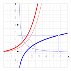
The thick blue curve and the thick red curve are inverse to each other. A thin curve is the derivative of the same colored thick curve. Inverse function rule:
f ( x ) = 1 [ f 1 ] ( f ( x ) ) {\displaystyle {\color {CornflowerBlue}{f'}}(x)={\frac {1}{{\color {Salmon}{\left[f^{-1}\right]'}}({\color {Blue}{f}}(x))}}}

Example for arbitrary x 0 5.8 {\displaystyle x_{0}\approx 5.8} :
f ( x 0 ) = 1 4 {\displaystyle {\color {CornflowerBlue}{f'}}(x_{0})={\frac {1}{4}}}
[ f 1 ] ( f ( x 0 ) ) = 4   {\displaystyle {\color {Salmon}{\left[f^{-1}\right]'}}({\color {Blue}{f}}(x_{0}))=4~} source ↗

In calculus, the inverse function rule is a formula that expresses the derivative of the inverse of a bijective and differentiable function f in terms of the derivative of f. More precisely, if the inverse of f {\displaystyle f} is denoted as f 1 {\displaystyle f^{-1}} , where f 1 ( y ) = x {\displaystyle f^{-1}(y)=x} if and only if f ( x ) = y {\displaystyle f(x)=y} , then the inverse function rule is, in Lagrange's notation,

[ f 1 ] ( y ) = 1 f ( f 1 ( y ) ) . {\displaystyle \left[f^{-1}\right]'(y)={\frac {1}{f'\left(f^{-1}(y)\right)}}.}

This formula holds in general whenever f {\displaystyle f} is continuous and injective on an interval I, with f {\displaystyle f} being differentiable at f 1 ( y ) {\displaystyle f^{-1}(y)} ( I {\displaystyle \in I} ) and where f ( f 1 ( y ) ) 0 {\displaystyle f'(f^{-1}(y))\neq 0} . The same formula is also equivalent to the expression

D [ f 1 ] = 1 ( D f ) ( f 1 ) , {\displaystyle {\mathcal {D}}\left[f^{-1}\right]={\frac {1}{({\mathcal {D}}f)\circ \left(f^{-1}\right)}},}

where D {\displaystyle {\mathcal {D}}} denotes the unary derivative operator (on the space of functions) and {\displaystyle \circ } denotes function composition.

Geometrically, a function and inverse function have graphs that are reflections, in the line y = x {\displaystyle y=x} . This reflection operation turns the gradient of any line into its reciprocal.1

Assuming that f {\displaystyle f} has an inverse in a neighbourhood of x {\displaystyle x} and that its derivative at that point is non-zero, its inverse is guaranteed to be differentiable at x {\displaystyle x} and have a derivative given by the above formula.

The inverse function rule may also be expressed in Leibniz's notation. As that notation suggests,

d x d y d y d x = 1. {\displaystyle {\frac {dx}{dy}}\,{\frac {dy}{dx}}=1.}

This relation is obtained by differentiating the equation f 1 ( y ) = x {\displaystyle f^{-1}(y)=x} in terms of x and applying the chain rule, yielding that:

d x d y d y d x = d x d x {\displaystyle {\frac {dx}{dy}}\,{\frac {dy}{dx}}={\frac {dx}{dx}}}

considering that the derivative of x with respect to x is 1.

Derivation

Let f {\displaystyle f} be an invertible (bijective) function, let x {\displaystyle x} be in the domain of f {\displaystyle f} , and let y = f ( x ) . {\displaystyle y=f(x).} Let g = f 1 . {\displaystyle g=f^{-1}.} So, f ( g ( y ) ) = y . {\displaystyle f(g(y))=y.} Differentiating this equation with respect to y {\displaystyle y} , and using the chain rule, one gets

f ( g ( y ) ) g ( y ) = 1. {\displaystyle f'(g(y))\cdot g'(y)=1.}

That is,

g ( y ) = 1 f ( g ( y ) ) {\displaystyle g'(y)={\frac {1}{f'(g(y))}}}

or

[ f 1 ] ( y ) = 1 f ( f 1 ( y ) ) . {\displaystyle \left[f^{-1}\right]^{\prime }(y)={\frac {1}{f^{\prime }(f^{-1}(y))}}.}

Examples

  • y = x 2 {\displaystyle y=x^{2}} (for positive x) has inverse x = y {\displaystyle x={\sqrt {y}}} .
d y d x = 2 x         ;         d x d y = 1 2 y = 1 2 x {\displaystyle {\frac {dy}{dx}}=2x{\mbox{ }}{\mbox{ }}{\mbox{ }}{\mbox{ }};{\mbox{ }}{\mbox{ }}{\mbox{ }}{\mbox{ }}{\frac {dx}{dy}}={\frac {1}{2{\sqrt {y}}}}={\frac {1}{2x}}}
d y d x d x d y = 2 x 1 2 x = 1. {\displaystyle {\frac {dy}{dx}}\,{\frac {dx}{dy}}=2x\cdot {\frac {1}{2x}}=1.}

At x = 0 {\displaystyle x=0} , however, there is a problem: the graph of the square root function becomes vertical, corresponding to a horizontal tangent for the square function.

  • y = e x {\displaystyle y=e^{x}} (for real x) has inverse x = ln y {\displaystyle x=\ln {y}} (for positive y {\displaystyle y} )
d y d x = e x         ;         d x d y = 1 y = e x {\displaystyle {\frac {dy}{dx}}=e^{x}{\mbox{ }}{\mbox{ }}{\mbox{ }}{\mbox{ }};{\mbox{ }}{\mbox{ }}{\mbox{ }}{\mbox{ }}{\frac {dx}{dy}}={\frac {1}{y}}=e^{-x}}
d y d x d x d y = e x e x = 1. {\displaystyle {\frac {dy}{dx}}\,{\frac {dx}{dy}}=e^{x}e^{-x}=1.}

Additional properties

f 1 ( y ) = 1 f ( f 1 ( y ) ) d y + C . {\displaystyle {f^{-1}}(y)=\int {\frac {1}{f'({f^{-1}}(y))}}\,{dy}+C.}
This is only useful if the integral exists. In particular we need f ( x ) {\displaystyle f'(x)} to be non-zero across the range of integration.
It follows that a function that has a continuous derivative has an inverse in a neighbourhood of every point where the derivative is non-zero. This need not be true if the derivative is not continuous.
  • Another very interesting and useful property is the following:
f 1 ( y ) d y = y f 1 ( y ) F ( f 1 ( y ) ) + C {\displaystyle \int f^{-1}(y)\,{dy}=yf^{-1}(y)-F(f^{-1}(y))+C}
where F {\displaystyle F} denotes the antiderivative of f {\displaystyle f} .
  • The inverse of the derivative of f(x) is also of interest, as it is used in showing the convexity of the Legendre transform.

Let z = f ( x ) {\displaystyle z=f'(x)} then we have, assuming f ( x ) 0 {\displaystyle f''(x)\neq 0} : d d z [ f ] 1 ( z ) = 1 f ( x ) {\displaystyle {\frac {d}{dz}}\left[f'\right]^{-1}(z)={\frac {1}{f''(x)}}} This can be shown using the previous notation y = f ( x ) {\displaystyle y=f(x)} . Then we have:

f ( x ) = d y d x = d y d z d z d x = d y d z f ( x ) d y d z = f ( x ) f ( x ) {\displaystyle f'(x)={\frac {dy}{dx}}={\frac {dy}{dz}}{\frac {dz}{dx}}={\frac {dy}{dz}}f''(x)\Rightarrow {\frac {dy}{dz}}={\frac {f'(x)}{f''(x)}}} Therefore:
d d z [ f ] 1 ( z ) = d x d z = d y d z d x d y = f ( x ) f ( x ) 1 f ( x ) = 1 f ( x ) {\displaystyle {\frac {d}{dz}}[f']^{-1}(z)={\frac {dx}{dz}}={\frac {dy}{dz}}{\frac {dx}{dy}}={\frac {f'(x)}{f''(x)}}{\frac {1}{f'(x)}}={\frac {1}{f''(x)}}}

By induction, we can generalize this result for any integer n 1 {\displaystyle n\geq 1} , with z = f ( n ) ( x ) {\displaystyle z=f^{(n)}(x)} , the nth derivative of f(x), and y = f ( n 1 ) ( x ) {\displaystyle y=f^{(n-1)}(x)} , assuming f ( i ) ( x ) 0  for  0 < i n + 1 {\displaystyle f^{(i)}(x)\neq 0{\text{ for }}0<i\leq n+1} :

d d z [ f ( n ) ] 1 ( z ) = 1 f ( n + 1 ) ( x ) {\displaystyle {\frac {d}{dz}}\left[f^{(n)}\right]^{-1}(z)={\frac {1}{f^{(n+1)}(x)}}}

Higher order derivatives

The chain rule given above is obtained by differentiating the identity f 1 ( y ) = x {\displaystyle f^{-1}(y)=x} with respect to y, where y = f ( x ) {\displaystyle y=f(x)} . One can continue the same process for higher derivatives. Differentiating the identity twice with respect to x, one obtains

d 2 y d x 2 d x d y + d d x ( d x d y ) ( d y d x ) = 0 , {\displaystyle {\frac {d^{2}y}{dx^{2}}}\,{\frac {dx}{dy}}+{\frac {d}{dx}}\left({\frac {dx}{dy}}\right)\,\left({\frac {dy}{dx}}\right)=0,}

that is simplified further by the chain rule as

d 2 y d x 2 d x d y + d 2 x d y 2 ( d y d x ) 2 = 0. {\displaystyle {\frac {d^{2}y}{dx^{2}}}\,{\frac {dx}{dy}}+{\frac {d^{2}x}{dy^{2}}}\,\left({\frac {dy}{dx}}\right)^{2}=0.}

Replacing the first derivative, using the identity obtained earlier, we get

d 2 y d x 2 = d 2 x d y 2 ( d y d x ) 3 {\displaystyle {\frac {d^{2}y}{dx^{2}}}=-{\frac {d^{2}x}{dy^{2}}}\,\left({\frac {dy}{dx}}\right)^{3}}

which implies

d 2 x d y 2 = d 2 y / d x 2 ( d y / d x ) 3 . {\displaystyle {\frac {d^{2}x}{dy^{2}}}=-{\frac {d^{2}y/dx^{2}}{\left(dy/dx\right)^{3}}}.}

Similarly for the third derivative we have

d 3 y d x 3 = d 3 x d y 3 ( d y d x ) 4 3 d 2 x d y 2 d 2 y d x 2 ( d y d x ) 2 . {\displaystyle {\frac {d^{3}y}{dx^{3}}}=-{\frac {d^{3}x}{dy^{3}}}\,\left({\frac {dy}{dx}}\right)^{4}-3{\frac {d^{2}x}{dy^{2}}}\,{\frac {d^{2}y}{dx^{2}}}\,\left({\frac {dy}{dx}}\right)^{2}.}

Using the formula for the second derivative, we get

d 3 y d x 3 = d 3 x d y 3 ( d y d x ) 4 + 3 ( d 2 y d x 2 ) 2 ( d y d x ) 1 {\displaystyle {\frac {d^{3}y}{dx^{3}}}=-{\frac {d^{3}x}{dy^{3}}}\,\left({\frac {dy}{dx}}\right)^{4}+3\left({\frac {d^{2}y}{dx^{2}}}\right)^{2}\,\left({\frac {dy}{dx}}\right)^{-1}}

which implies

d 3 x d y 3 = d 3 y / d x 3 ( d y / d x ) 4 + 3 ( d 2 y / d x 2 ) 2 ( d y / d x ) 5 . {\displaystyle {\frac {d^{3}x}{dy^{3}}}=-{\frac {d^{3}y/dx^{3}}{\left(dy/dx\right)^{4}}}+3{\frac {\left(d^{2}y/dx^{2}\right)^{2}}{\left(dy/dx\right)^{5}}}.}

These formulas can also be written using Lagrange's notation:

[ f 1 ] ( y ) = f ( f 1 ( y ) ) [ f ( f 1 ( y ) ) ] 3 , {\displaystyle \left[f^{-1}\right]''(y)=-{\frac {f''(f^{-1}(y))}{\left[f'(f^{-1}(y))\right]^{3}}},}
[ f 1 ] ( y ) = f ( f 1 ( y ) ) [ f ( f 1 ( y ) ) ] 4 + 3 [ f ( f 1 ( y ) ) ] 2 [ f ( f 1 ( y ) ) ] 5 . {\displaystyle \left[f^{-1}\right]'''(y)=-{\frac {f'''(f^{-1}(y))}{\left[f'(f^{-1}(y))\right]^{4}}}+3{\frac {\left[f''(f^{-1}(y))\right]^{2}}{\left[f'(f^{-1}(y))\right]^{5}}}.}

In general, higher order derivatives of an inverse function can be expressed with Faà di Bruno's formula. Alternatively, the nth derivative can be written succinctly as:

[ f 1 ] ( n ) ( y ) = [ ( 1 f ( t ) d d t ) n t ] t = f 1 ( y ) . {\displaystyle \left[f^{-1}\right]^{(n)}(y)=\left[\left({\frac {1}{f'(t)}}{\frac {d}{dt}}\right)^{n}t\right]_{t=f^{-1}(y)}.}

From this expression, one can also derive the nth-integration of inverse function with base-point a using Cauchy formula for repeated integration whenever f ( f 1 ( y ) ) = y {\displaystyle f(f^{-1}(y))=y} :

[ f 1 ] ( n ) ( y ) = 1 n ! ( f 1 ( a ) ( y a ) n + f 1 ( a ) f 1 ( y ) ( y f ( u ) ) n d u ) . {\displaystyle \left[f^{-1}\right]^{(-n)}(y)={\frac {1}{n!}}\left(f^{-1}(a)(y-a)^{n}+\int _{f^{-1}(a)}^{f^{-1}(y)}\left(y-f(u)\right)^{n}\,du\right).}

Example

  • y = e x {\displaystyle y=e^{x}} has the inverse x = ln y {\displaystyle x=\ln y} . Using the formula for the second derivative of the inverse function,
d y d x = d 2 y d x 2 = e x = y         ;         ( d y d x ) 3 = y 3 ; {\displaystyle {\frac {dy}{dx}}={\frac {d^{2}y}{dx^{2}}}=e^{x}=y{\mbox{ }}{\mbox{ }}{\mbox{ }}{\mbox{ }};{\mbox{ }}{\mbox{ }}{\mbox{ }}{\mbox{ }}\left({\frac {dy}{dx}}\right)^{3}=y^{3};}

so that

d 2 x d y 2 y 3 + y = 0         ;         d 2 x d y 2 = 1 y 2 , {\displaystyle {\frac {d^{2}x}{dy^{2}}}\,\cdot \,y^{3}+y=0{\mbox{ }}{\mbox{ }}{\mbox{ }}{\mbox{ }};{\mbox{ }}{\mbox{ }}{\mbox{ }}{\mbox{ }}{\frac {d^{2}x}{dy^{2}}}=-{\frac {1}{y^{2}}},}

which agrees with the direct calculation.

See also

See also

References

References

  1. "Derivatives of Inverse Functions". oregonstate.edu. Archived from the original on 2021-04-10. Retrieved 2019-07-26.
  • Marsden, Jerrold E.; Weinstein, Alan (1981). "Chapter 8: Inverse Functions and the Chain Rule". Calculus unlimited (PDF). Menlo Park, Calif.: Benjamin/Cummings Pub. Co. ISBN 0-8053-6932-5.