Giant component

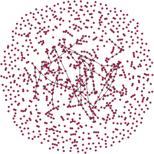
In network theory, a giant component is a connected component of a given random graph that contains a significant fraction of the entire graph's vertices.

More precisely, in graphs drawn randomly from a probability distribution over arbitrarily large graphs, a giant component is a connected component whose fraction of the overall number of vertices is bounded away from zero. In sufficiently dense graphs distributed according to the Erdős–Rényi model, a giant component exists with high probability.

Giant components are a prominent feature of the Erdős–Rényi model (ER) of random graphs, in which each possible edge connecting pairs of a given set of n vertices is present, independently of the other edges, with probability p. In this model, if ${\displaystyle p\leq {\frac {1-\epsilon }{n}}}$ for any constant ${\displaystyle \epsilon >0}$, then with high probability (in the limit as ${\displaystyle n}$ goes to infinity) all connected components of the graph have size O(log n), and there is no giant component. However, for ${\displaystyle p\geq {\frac {1+\epsilon }{n}}}$ there is with high probability a single giant component, with all other components having size O(log n). For ${\displaystyle p=p_{c}={\frac {1}{n}}}$, intermediate between these two possibilities, the number of vertices in the largest component of the graph, ${\displaystyle P_{\inf }}$ is with high probability proportional to ${\displaystyle n^{2/3}}$.¹

Giant component is also important in percolation theory.¹² When a fraction of nodes, ${\displaystyle q=1-p}$, is removed randomly from an ER network of degree ${\displaystyle \langle k\rangle }$, there exists a critical threshold, ${\displaystyle p_{c}={\frac {1}{\langle k\rangle }}}$. Above ${\displaystyle p_{c}}$ there exists a giant component (largest cluster) of size, ${\displaystyle P_{\inf }}$. ${\displaystyle P_{\inf }}$ fulfills, ${\displaystyle P_{\inf }=p(1-\exp(-\langle k\rangle P_{\inf }))}$. For ${\displaystyle p<p_{c}}$ the solution of this equation is ${\displaystyle P_{\inf }=0}$, i.e., there is no giant component.

At ${\displaystyle p_{c}}$, the distribution of cluster sizes behaves as a power law, ${\displaystyle n(s)}$~${\displaystyle s^{-5/2}}$ which is a feature of phase transition.

Alternatively, if one adds randomly selected edges one at a time, starting with an empty graph, then it is not until approximately ${\displaystyle n/2}$ edges have been added that the graph contains a large component, and soon after that the component becomes giant. More precisely, when t edges have been added, for values of t close to but larger than ${\displaystyle n/2}$, the size of the giant component is approximately ${\displaystyle 4t-2n}$.¹ However, according to the coupon collector's problem, ${\displaystyle \Theta (n\log n)}$ edges are needed in order to have high probability that the whole random graph is connected.

A similar sharp threshold between parameters that lead to graphs with all components small and parameters that lead to a giant component also occurs in tree-like random graphs with non-uniform degree distributions ${\displaystyle P(k)}$. The degree distribution does not define a graph uniquely. However, under the assumption that in all respects other than their degree distribution, the graphs are treated as entirely random, many results on finite/infinite-component sizes are known. In this model, the existence of the giant component depends only on the first two (mixed) moments of the degree distribution. Let a randomly chosen vertex have degree ${\displaystyle k}$, then the giant component exists³ if and only if$${\displaystyle \langle k^{2}\rangle -2\langle k\rangle >0.}$$This is known as the Molloy and Reed condition.⁴ The first moment of ${\displaystyle P(k)}$ is the mean degree of the network. In general, the ${\displaystyle n}$-th moment is defined as ${\displaystyle \langle k^{n}\rangle =\mathbb {E} [k^{n}]=\sum k^{n}P(k)}$.

When there is no giant component, the expected size of the small component can also be determined by the first and second moments and it is ${\displaystyle 1+{\frac {\langle k\rangle ^{2}}{2\langle k\rangle +\langle k^{2}\rangle }}.}$ However, when there is a giant component, the size of the giant component is more tricky to evaluate.²

Similar expressions are also valid for directed graphs, in which case the degree distribution is two-dimensional.⁵ There are three types of connected components in directed graphs. For a randomly chosen vertex:

1. out-component is a set of vertices that can be reached by recursively following all out-edges forward;
2. in-component is a set of vertices that can be reached by recursively following all in-edges backward;
3. weak component is a set of vertices that can be reached by recursively following all edges regardless of their direction.

Let a randomly chosen vertex has ${\displaystyle k_{\text{in}}}$ in-edges and ${\displaystyle k_{\text{out}}}$ out edges. By definition, the average number of in- and out-edges coincides so that ${\displaystyle c=\mathbb {E} [k_{\text{in}}]=\mathbb {E} [k_{\text{out}}]}$. If ${\displaystyle G_{0}(x)=\textstyle \sum _{k}\displaystyle P(k)x^{k}}$ is the generating function of the degree distribution ${\displaystyle P(k)}$ for an undirected network, then ${\displaystyle G_{1}(x)}$ can be defined as ${\displaystyle G_{1}(x)=\textstyle \sum _{k}\displaystyle {\frac {k}{\langle k\rangle }}P(k)x^{k-1}}$. For directed networks, generating function assigned to the joint probability distribution ${\displaystyle P(k_{in},k_{out})}$ can be written with two valuables ${\displaystyle x}$ and ${\displaystyle y}$ as: ${\displaystyle {\mathcal {G}}(x,y)=\sum _{k_{in},k_{out}}\displaystyle P({k_{in},k_{out}})x^{k_{in}}y^{k_{out}}}$, then one can define ${\displaystyle g(x)={\frac {1}{c}}{\partial {\mathcal {G}} \over \partial x}\vert _{y=1}}$ and ${\displaystyle f(y)={\frac {1}{c}}{\partial {\mathcal {G}} \over \partial y}\vert _{x=1}}$. The criteria for giant component existence in directed and undirected random graphs are given in the table below:

Type	Criteria
undirected: giant component	${\displaystyle \mathbb {E} [k^{2}]-2\mathbb {E} [k]>0}$,3 or ${\displaystyle G'_{1}(1)=1}$5
directed: giant in/out-component	${\displaystyle \mathbb {E} [k_{\text{in}}k_{out}]-\mathbb {E} [k_{\text{in}}]>0}$,5 or ${\displaystyle g'_{1}(1)=f'_{1}(1)=1}$5
directed: giant weak component	${\displaystyle 2\mathbb {E} [k_{\text{in}}]\mathbb {E} [k_{\text{in}}k_{\text{out}}]-\mathbb {E} [k_{\text{in}}]\mathbb {E} [k_{\text{out}}^{2}]-\mathbb {E} [k_{\text{in}}]\mathbb {E} [k_{\text{in}}^{2}]+\mathbb {E} [k_{\text{in}}^{2}]\mathbb {E} [k_{\text{out}}^{2}]-\mathbb {E} [k_{\text{in}}k_{\text{out}}]^{2}>0}$6

References

- Bollobás, Béla (2001), "6. The Evolution of Random Graphs—The Giant Component", Random Graphs, Cambridge studies in advanced mathematics, vol. 73 (2nd ed.), Cambridge University Press, pp. 130–159, ISBN 978-0-521-79722-1.
- Newman, M. E. J. (2010). Networks: an introduction. New York: Oxford University Press. OCLC 456837194.
- Molloy, Michael; Reed, Bruce (1995). "A critical point for random graphs with a given degree sequence". Random Structures & Algorithms. 6 (2–3): 161–180. doi:10.1002/rsa.3240060204. ISSN 1042-9832.
- Molloy, Michael; Reed, Bruce (March 1995). "A critical point for random graphs with a given degree sequence". Random Structures & Algorithms. 6 (2–3): 161–180. doi:10.1002/rsa.3240060204. ISSN 1042-9832.
- Newman, M. E. J.; Strogatz, S. H.; Watts, D. J. (2001-07-24). "Random graphs with arbitrary degree distributions and their applications". Physical Review E. 64 (2) 026118. arXiv:cond-mat/0007235. Bibcode:2001PhRvE..64b6118N. doi:10.1103/physreve.64.026118. ISSN 1063-651X. PMID 11497662.
- Kryven, Ivan (2016-07-27). "Emergence of the giant weak component in directed random graphs with arbitrary degree distributions". Physical Review E. 94 (1) 012315. arXiv:1607.03793. Bibcode:2016PhRvE..94a2315K. doi:10.1103/physreve.94.012315. ISSN 2470-0045. PMID 27575156. S2CID 206251373.