F-distribution

Fisher–Snedecor
Probability density function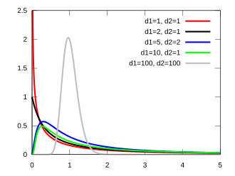
Cumulative distribution function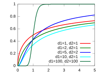
Parameters	d1, d2 > 0 deg. of freedom
Support	x ∈ (0, +∞) if d1 = 1, otherwise x ∈ [0, +∞)
PDF	${\displaystyle {\frac {\sqrt {\frac {(d_{1}x)^{d_{1}}d_{2}^{d_{2}}}{(d_{1}x+d_{2})^{d_{1}+d_{2}}}}}{x\,\mathrm {B} \!\left({\frac {d_{1}}{2}},{\frac {d_{2}}{2}}\right)}}}$
CDF	${\displaystyle I_{\frac {d_{1}x}{d_{1}x+d_{2}}}\left({\tfrac {d_{1}}{2}},{\tfrac {d_{2}}{2}}\right)}$
Mean	${\displaystyle {\frac {d_{2}}{d_{2}-2}}}$ for d2 > 2
Mode	${\displaystyle {\frac {d_{1}-2}{d_{1}}}\;{\frac {d_{2}}{d_{2}+2}}}$ for d1 > 2
Variance	${\displaystyle {\frac {2\,d_{2}^{2}\,(d_{1}+d_{2}-2)}{d_{1}(d_{2}-2)^{2}(d_{2}-4)}}}$ for d2 > 4
Skewness	${\displaystyle {\frac {(2d_{1}+d_{2}-2){\sqrt {8(d_{2}-4)}}}{(d_{2}-6){\sqrt {d_{1}(d_{1}+d_{2}-2)}}}}}$ for d2 > 6
Excess kurtosis	see text
Entropy	${\displaystyle {\begin{aligned}&\ln \Gamma {\left({\tfrac {d_{1}}{2}}\right)}+\ln \Gamma {\left({\tfrac {d_{2}}{2}}\right)}-\ln \Gamma {\left({\tfrac {d_{1}+d_{2}}{2}}\right)}\\&+\left(1-{\tfrac {d_{1}}{2}}\right)\psi {\left(1+{\tfrac {d_{1}}{2}}\right)}\\&-\left(1+{\tfrac {d_{2}}{2}}\right)\psi {\left(1+{\tfrac {d_{2}}{2}}\right)}\\&+\left({\tfrac {d_{1}+d_{2}}{2}}\right)\psi {\left({\tfrac {d_{1}+d_{2}}{2}}\right)}+\ln {\frac {d_{2}}{d_{1}}}\end{aligned}}}$1
MGF	does not exist, raw moments defined in text and in 23
CF	see text

In probability theory and statistics, the F-distribution or F-ratio, also known as Snedecor's F distribution or the Fisher–Snedecor distribution (after Ronald Fisher and George W. Snedecor), is a continuous probability distribution that arises frequently as the null distribution of a test statistic, most notably in the analysis of variance (ANOVA) and other F-tests.²³⁴⁵

The F-distribution with ⁠${\displaystyle d_{1}}$⁠ and ⁠${\displaystyle d_{2}}$⁠ degrees of freedom is the distribution of $${\displaystyle X={\frac {U_{1}/d_{1}}{U_{2}/d_{2}}}}$$

where ${\textstyle U_{1}}$ and ${\textstyle U_{2}}$ are independent random variables with chi-square distributions with respective degrees of freedom ⁠${\displaystyle d_{1}}$⁠ and ⁠${\displaystyle d_{2}}$⁠.

It can be shown to follow that the probability density function (PDF) for ⁠${\displaystyle X}$⁠ is given by $${\displaystyle {\begin{aligned}f(x;d_{1},d_{2})&={\frac {\sqrt {\frac {(d_{1}x)^{d_{1}}\,\,d_{2}^{d_{2}}}{(d_{1}x+d_{2})^{d_{1}+d_{2}}}}}{x\operatorname {B} \left({\frac {d_{1}}{2}},{\frac {d_{2}}{2}}\right)}}\\[5pt]&={\frac {\left({\frac {d_{1}}{d_{2}}}\right)^{\frac {d_{1}}{2}}{x{\vphantom {\left({d_{1} \over d_{2}}\right)}}}^{{\frac {d_{1}}{2}}-1}\left(1+{\frac {d_{1}}{d_{2}}}\,x\right)^{-{\frac {d_{1}+d_{2}}{2}}}}{\operatorname {B} \left({\frac {d_{1}}{2}},{\frac {d_{2}}{2}}\right)}}\end{aligned}}}$$

for real ⁠${\displaystyle x>0}$⁠. Here ${\displaystyle \mathrm {B} }$ is the beta function. In many applications, the parameters ⁠${\displaystyle d_{1}}$⁠ and ⁠${\displaystyle d_{2}}$⁠ are positive integers, but the distribution is well-defined for positive real values of these parameters.

The cumulative distribution function is $${\displaystyle F(x;d_{1},d_{2})=I_{\frac {d_{1}x}{(d_{1}x+d_{2})}}\left({\tfrac {d_{1}}{2}},{\tfrac {d_{2}}{2}}\right),}$$

where ⁠${\displaystyle I_{x}(a,b)}$⁠ is the regularized incomplete beta function.

The expectation, variance, and other details about the F-distribution ⁠${\displaystyle F(d_{1},d_{2})}$⁠ are given in the sidebox; for ⁠${\displaystyle d_{2}>8}$⁠, the excess kurtosis is $${\displaystyle \gamma _{2}=12{\frac {d_{1}(5d_{2}-22)(d_{1}+d_{2}-2)+(d_{2}-4)(d_{2}-2)^{2}}{d_{1}(d_{2}-6)(d_{2}-8)(d_{1}+d_{2}-2)}}.}$$

The k-th moment of an ⁠${\displaystyle F(d_{1},d_{2})}$⁠ distribution exists and is finite only when ⁠${\displaystyle 2k<d_{2}}$⁠ and it is equal to⁶

$${\displaystyle \mu _{X}(k)=\left({\frac {d_{2}}{d_{1}}}\right)^{k}{\frac {\Gamma \left({\tfrac {d_{1}}{2}}+k\right)}{\Gamma \left({\tfrac {d_{1}}{2}}\right)}}{\frac {\Gamma \left({\tfrac {d_{2}}{2}}-k\right)}{\Gamma \left({\tfrac {d_{2}}{2}}\right)}}.}$$

The F-distribution is a particular parametrization of the beta prime distribution, which is also called the beta distribution of the second kind.

The characteristic function is listed incorrectly in many standard references (e.g.,³). The correct expression ⁷ is

$${\displaystyle \varphi _{d_{1},d_{2}}^{F}(s)={\frac {\Gamma {\left({\frac {d_{1}+d_{2}}{2}}\right)}}{\Gamma {\left({\tfrac {d_{2}}{2}}\right)}}}U\!\left({\frac {d_{1}}{2}},1-{\frac {d_{2}}{2}},-{\frac {d_{2}}{d_{1}}}\imath s\right)}$$

where ⁠${\displaystyle U(a,b,z)}$⁠ is the confluent hypergeometric function of the second kind.

In instances where the F-distribution is used, for example in the analysis of variance, independence of ⁠${\displaystyle U_{1}}$⁠ and ⁠${\displaystyle U_{2}}$⁠ (defined above) might be demonstrated by applying Cochran's theorem.

Equivalently, since the chi-squared distribution is the sum of squares of independent standard normal random variables, the random variable of the F-distribution may also be written $${\displaystyle X={\frac {s_{1}^{2}}{\sigma _{1}^{2}}}\div {\frac {s_{2}^{2}}{\sigma _{2}^{2}}},}$$

where ${\textstyle s_{1}^{2}={\frac {S_{1}^{2}}{d_{1}}}}$ and ⁠${\displaystyle \textstyle s_{2}^{2}={\frac {S_{2}^{2}}{d_{2}}}}$⁠, ${\displaystyle S_{1}^{2}}$ is the sum of squares of ${\displaystyle d_{1}}$ random variables from normal distribution ${\displaystyle N(0,\sigma _{1}^{2})}$ and ${\displaystyle S_{2}^{2}}$ is the sum of squares of ${\displaystyle d_{2}}$ random variables from normal distribution ⁠${\displaystyle N(0,\sigma _{2}^{2})}$⁠.

In a frequentist context, a scaled F-distribution therefore gives the probability ⁠${\displaystyle \textstyle p(s_{1}^{2}/s_{2}^{2}\mid \sigma _{1}^{2},\sigma _{2}^{2})}$⁠, with the F-distribution itself, without any scaling, applying where ${\displaystyle \sigma _{1}^{2}}$ is being taken equal to ⁠${\displaystyle \sigma _{2}^{2}}$⁠. This is the context in which the F-distribution most generally appears in F-tests: where the null hypothesis is that two independent normal variances are equal, and the observed sums of some appropriately selected squares are then examined to see whether their ratio is significantly incompatible with this null hypothesis.

The quantity ${\displaystyle X}$ has the same distribution in Bayesian statistics, if an uninformative rescaling-invariant Jeffreys prior is taken for the prior probabilities of ${\displaystyle \sigma _{1}^{2}}$ and ⁠${\displaystyle \sigma _{2}^{2}}$⁠.⁸ In this context, a scaled F-distribution thus gives the posterior probability ⁠${\displaystyle \textstyle p(\sigma _{2}^{2}/\sigma _{1}^{2}\mid s_{1}^{2},s_{2}^{2})}$⁠, where the observed sums ${\displaystyle s_{1}^{2}}$ and ${\displaystyle s_{2}^{2}}$ are now taken as known.

• If ${\displaystyle X\sim \chi _{d_{1}}^{2}}$ and ${\displaystyle Y\sim \chi _{d_{2}}^{2}}$ (Chi squared distribution) are independent, then ⁠${\displaystyle \textstyle {\frac {X/d_{1}}{Y/d_{2}}}\sim \mathrm {F} (d_{1},d_{2})}$⁠.
• If ${\displaystyle X_{k}\sim \Gamma (\alpha _{k},\beta _{k})\,}$ (Gamma distribution) are independent, then ⁠${\displaystyle \textstyle {\frac {\alpha _{2}\beta _{1}X_{1}}{\alpha _{1}\beta _{2}X_{2}}}\sim \mathrm {F} (2\alpha _{1},2\alpha _{2})}$⁠.
• If ${\textstyle X\sim \operatorname {Beta} \left({d_{1} \over 2},{d_{2} \over 2}\right)}$ (Beta distribution) then ⁠${\displaystyle \textstyle {\frac {d_{2}X}{d_{1}(1-X)}}\sim \operatorname {F} (d_{1},d_{2})}$⁠.
  • Equivalently, if ⁠${\displaystyle X\sim F(d_{1},d_{2})}$⁠, then ⁠${\displaystyle \textstyle {\frac {d_{1}X/d_{2}}{1+d_{1}X/d_{2}}}\sim \operatorname {Beta} \left({d_{1} \over 2},{d_{2} \over 2}\right)}$⁠.
• If ⁠${\displaystyle X\sim F(d_{1},d_{2})}$⁠, then ${\textstyle {\frac {d_{1}}{d_{2}}}X}$ has a beta prime distribution: ⁠${\displaystyle \textstyle {\frac {d_{1}}{d_{2}}}X\sim \operatorname {\beta ^{\prime }} \left({\tfrac {d_{1}}{2}},{\tfrac {d_{2}}{2}}\right)}$⁠.
• If ${\displaystyle X\sim F(d_{1},d_{2})}$ then ${\textstyle Y=\lim _{d_{2}\to \infty }d_{1}X}$ has the chi-squared distribution ⁠${\displaystyle \chi _{d_{1}}^{2}}$⁠.
• ${\displaystyle F(d_{1},d_{2})}$ is equivalent to the scaled Hotelling's T-squared distribution ⁠${\displaystyle \textstyle {\frac {d_{2}}{d_{1}(d_{1}+d_{2}-1)}}\operatorname {T} ^{2}(d_{1},d_{1}+d_{2}-1)}$⁠.
• If ${\displaystyle X\sim F(d_{1},d_{2})}$ then ⁠${\displaystyle X^{-1}\sim F(d_{2},d_{1})}$⁠.
• If ⁠${\displaystyle X\sim t_{(n)}}$⁠ – Student's t-distribution – then: $${\displaystyle {\begin{aligned}X^{2}&\sim \operatorname {F} (1,n),\\X^{-2}&\sim \operatorname {F} (n,1).\end{aligned}}}$$
• F-distribution is a special case of type 6 Pearson distribution.
• If ${\displaystyle X}$ and ${\displaystyle Y}$ are independent, with ⁠${\displaystyle X,Y\sim \operatorname {Laplace} (\mu ,b)}$⁠ (Laplace distribution), then $${\displaystyle {\frac {|X-\mu |}{|Y-\mu |}}\sim \operatorname {F} (2,2).}$$
• If ${\displaystyle X\sim F(n,m)}$ then ${\displaystyle {\tfrac {\log {X}}{2}}\sim \operatorname {FisherZ} (n,m)}$ (Fisher's z-distribution).
• The noncentral F-distribution simplifies to the F-distribution if ⁠${\displaystyle \lambda =0}$⁠.
• The doubly noncentral F-distribution simplifies to the F-distribution if ⁠${\displaystyle \lambda _{1}=\lambda _{2}=0}$⁠
• If ${\displaystyle \operatorname {Q} _{X}(p)}$ is the quantile ⁠${\displaystyle p}$⁠ for ${\displaystyle X\sim F(d_{1},d_{2})}$ and ${\displaystyle \operatorname {Q} _{Y}(1-p)}$ is the quantile ${\displaystyle 1-p}$ for ⁠${\displaystyle Y\sim F(d_{2},d_{1})}$⁠, then $${\displaystyle \operatorname {Q} _{X}(p)={\frac {1}{\operatorname {Q} _{Y}(1-p)}}.}$$
• F-distribution is an instance of ratio distributions.
• W-distribution is a unique parametrization of F-distribution.

References

- Lazo, A.V.; Rathie, P. (1978). "On the entropy of continuous probability distributions". IEEE Transactions on Information Theory. 24 (1). IEEE: 120–122. doi:10.1109/tit.1978.1055832.
- Johnson, Norman Lloyd; Samuel Kotz; N. Balakrishnan (1995). Continuous Univariate Distributions, Volume 2 (Section 27) (2nd ed.). Wiley. ISBN 0-471-58494-0.
- Abramowitz, Milton; Stegun, Irene Ann, eds. (1983) [June 1964]. "Chapter 26". Handbook of Mathematical Functions with Formulas, Graphs, and Mathematical Tables. Applied Mathematics Series. Vol. 55 (Ninth reprint with additional corrections of tenth original printing with corrections (December 1972); first ed.). Washington D.C.; New York: United States Department of Commerce, National Bureau of Standards; Dover Publications. p. 946. ISBN 978-0-486-61272-0. LCCN 64-60036. MR 0167642. LCCN 65-12253.
- NIST (2006). Engineering Statistics Handbook – F Distribution
- Mood, Alexander; Franklin A. Graybill; Duane C. Boes (1974). Introduction to the Theory of Statistics (Third ed.). McGraw-Hill. pp. 246–249. ISBN 0-07-042864-6.
- Taboga, Marco. "The F distribution".
- Phillips, P. C. B. (1982) "The true characteristic function of the F distribution," Biometrika, 69: 261–264 JSTOR 2335882
- Box, G. E. P.; Tiao, G. C. (1973). Bayesian Inference in Statistical Analysis. Addison-Wesley. p. 110. ISBN 0-201-00622-7.
External links