Article · Wikipedia archive · Last revised Jun 3, 2026

Cramer's rule

In linear algebra, Cramer's rule is an explicit formula for the solution of a system of linear equations with as many equations as unknowns, valid whenever the system has a unique solution. It expresses the solution in terms of the determinants of the (square) coefficient matrix and of matrices obtained from it by replacing one column by the column vector of right-sides of the equations. It is named after Gabriel Cramer, who published the rule for an arbitrary number of unknowns in 1750, although Colin Maclaurin also published special cases of the rule in 1748, and possibly knew of it as early as 1729.

Last revised
Jun 3, 2026
Read time
≈ 27 min
Length
6,226 w
Citations
15
Source

In linear algebra, Cramer's rule is an explicit formula for the solution of a system of linear equations with as many equations as unknowns, valid whenever the system has a unique solution. It expresses the solution in terms of the determinants of the (square) coefficient matrix and of matrices obtained from it by replacing one column by the column vector of right-sides of the equations. It is named after Gabriel Cramer, who published the rule for an arbitrary number of unknowns in 1750,12 although Colin Maclaurin also published special cases of the rule in 1748,3 and possibly knew of it as early as 1729.456

General case

Consider a system of n linear equations for n unknowns, represented in matrix multiplication form as follows:

A x = b {\displaystyle A\mathbf {x} =\mathbf {b} }

where the n × n matrix A has a nonzero determinant, and the vector x = ( x 1 , , x n ) T {\displaystyle \mathbf {x} =(x_{1},\ldots ,x_{n})^{\mathsf {T}}} is the column vector of the variables. Then the theorem states that in this case the system has a unique solution, whose individual values for the unknowns are given by:

x i = det ( A i ) det ( A ) i = 1 , , n {\displaystyle x_{i}={\frac {\det(A_{i})}{\det(A)}}\qquad i=1,\ldots ,n}

where A i {\displaystyle A_{i}} is the matrix formed by replacing the i-th column of A by the column vector b.

A more general version of Cramer's rule7 considers the matrix equation

A X = B {\displaystyle AX=B}

where the n × n matrix A has a nonzero determinant, and X, B are n × m matrices. Given sequences 1 i 1 < i 2 < < i k n {\displaystyle 1\leq i_{1}<i_{2}<\cdots <i_{k}\leq n} and 1 j 1 < j 2 < < j k m {\displaystyle 1\leq j_{1}<j_{2}<\cdots <j_{k}\leq m} , let X I , J {\displaystyle X_{I,J}} be the k × k submatrix of X with rows in I := ( i 1 , , i k ) {\displaystyle I:=(i_{1},\ldots ,i_{k})} and columns in J := ( j 1 , , j k ) {\displaystyle J:=(j_{1},\ldots ,j_{k})} . Let A B ( I , J ) {\displaystyle A_{B}(I,J)} be the n × n matrix formed by replacing the i s {\displaystyle i_{s}} column of A by the j s {\displaystyle j_{s}} column of B, for all s = 1 , , k {\displaystyle s=1,\ldots ,k} . Then

det X I , J = det ( A B ( I , J ) ) det ( A ) . {\displaystyle \det X_{I,J}={\frac {\det(A_{B}(I,J))}{\det(A)}}.}

In the case k = 1 {\displaystyle k=1} , this reduces to the normal Cramer's rule.

The rule holds for systems of equations with coefficients and unknowns in any field, not just in the real numbers.

Proof

The proof for Cramer's rule uses the following properties of the determinants: linearity with respect to any given column and the fact that the determinant is zero whenever two columns are equal, which is implied by the property that the sign of the determinant flips if you switch two columns.

Fix the index j of a column, and consider that the entries of the other columns have fixed values. This makes the determinant a function of the entries of the jth column. Linearity with respect to this column means that this function has the form

D j ( a 1 , j , , a n , j ) = C 1 , j a 1 , j + , C n , j a n , j , {\displaystyle D_{j}(a_{1,j},\ldots ,a_{n,j})=C_{1,j}a_{1,j}+\cdots ,C_{n,j}a_{n,j},}

where the C i , j {\displaystyle C_{i,j}} are coefficients that depend on the entries of A that are not in column j. So, one has

det ( A ) = D j ( a 1 , j , , a n , j ) = C 1 , j a 1 , j + , C n , j a n , j {\displaystyle \det(A)=D_{j}(a_{1,j},\ldots ,a_{n,j})=C_{1,j}a_{1,j}+\cdots ,C_{n,j}a_{n,j}}

(Laplace expansion provides a formula for computing the C i , j {\displaystyle C_{i,j}} but their expression is not important here.)

If the function D j {\displaystyle D_{j}} is applied to any other column k of A, then the result is the determinant of the matrix obtained from A by replacing column j by a copy of column k, so the resulting determinant is 0 (the case of two equal columns).

Now consider a system of n linear equations in n unknowns x 1 , , x n {\displaystyle x_{1},\ldots ,x_{n}} , whose coefficient matrix is A, with det(A) assumed to be nonzero:

a 11 x 1 + a 12 x 2 + + a 1 n x n = b 1 a 21 x 1 + a 22 x 2 + + a 2 n x n = b 2 a n 1 x 1 + a n 2 x 2 + + a n n x n = b n . {\displaystyle {\begin{matrix}a_{11}x_{1}+a_{12}x_{2}+\cdots +a_{1n}x_{n}&=&b_{1}\\a_{21}x_{1}+a_{22}x_{2}+\cdots +a_{2n}x_{n}&=&b_{2}\\&\vdots &\\a_{n1}x_{1}+a_{n2}x_{2}+\cdots +a_{nn}x_{n}&=&b_{n}.\end{matrix}}}

If one combines these equations by taking C1,j times the first equation, plus C2,j times the second, and so forth until Cn,j times the last, then for every k the resulting coefficient of xk becomes

D j ( a 1 , k , , a n , k ) . {\displaystyle D_{j}(a_{1,k},\ldots ,a_{n,k}).}

So, all coefficients become zero, except the coefficient of x j {\displaystyle x_{j}} that becomes det ( A ) . {\displaystyle \det(A).} Similarly, the constant coefficient becomes D j ( b 1 , , b n ) , {\displaystyle D_{j}(b_{1},\ldots ,b_{n}),} and the resulting equation is thus

det ( A ) x j = D j ( b 1 , , b n ) , {\displaystyle \det(A)x_{j}=D_{j}(b_{1},\ldots ,b_{n}),}

which gives the value of x j {\displaystyle x_{j}} as

x j = 1 det ( A ) D j ( b 1 , , b n ) . {\displaystyle x_{j}={\frac {1}{\det(A)}}D_{j}(b_{1},\ldots ,b_{n}).}

As, by construction, the numerator is the determinant of the matrix obtained from A by replacing column j by b, we get the expression of Cramer's rule as a necessary condition for a solution.

It remains to prove that these values for the unknowns form a solution. Let M be the n × n matrix that has the coefficients of D j {\displaystyle D_{j}} as jth row, for j = 1 , , n {\displaystyle j=1,\ldots ,n} (this is the adjugate matrix for A). Expressed in matrix terms, we have thus to prove that

x = 1 det ( A ) M b {\displaystyle \mathbf {x} ={\frac {1}{\det(A)}}M\mathbf {b} }

is a solution; that is, that

A ( 1 det ( A ) M ) b = b . {\displaystyle A\left({\frac {1}{\det(A)}}M\right)\mathbf {b} =\mathbf {b} .}

For that, it suffices to prove that

A ( 1 det ( A ) M ) = I n , {\displaystyle A\,\left({\frac {1}{\det(A)}}M\right)=I_{n},}

where I n {\displaystyle I_{n}} is the identity matrix.

The above properties of the functions D j {\displaystyle D_{j}} show that one has MA = det(A)In, and therefore,

( 1 det ( A ) M ) A = I n . {\displaystyle \left({\frac {1}{\det(A)}}M\right)\,A=I_{n}.}

This completes the proof, since a left inverse of a square matrix is also a right-inverse (see Invertible matrix theorem).

For other proofs, see below.

Finding inverse matrix

Let A be an n × n matrix with entries in a field F. Then

A adj ( A ) = adj ( A ) A = det ( A ) I {\displaystyle A\,\operatorname {adj} (A)=\operatorname {adj} (A)\,A=\det(A)I}

where adj(A) denotes the adjugate matrix, det(A) is the determinant, and I is the identity matrix. If det(A) is nonzero, then the inverse matrix of A is

A 1 = 1 det ( A ) adj ( A ) . {\displaystyle A^{-1}={\frac {1}{\det(A)}}\operatorname {adj} (A).}

This gives a formula for the inverse of A, provided det(A) ≠ 0. In fact, this formula works whenever F is a commutative ring, provided that det(A) is a unit. If det(A) is not a unit, then A is not invertible over the ring (it may be invertible over a larger ring in which some non-unit elements of F may be invertible).

Applications

Explicit formulas for small systems

Consider the linear system

{ a 1 x + b 1 y = c 1 a 2 x + b 2 y = c 2 {\displaystyle \left\{{\begin{matrix}a_{1}x+b_{1}y&={\color {red}c_{1}}\\a_{2}x+b_{2}y&={\color {red}c_{2}}\end{matrix}}\right.}

which in matrix format is

[ a 1 b 1 a 2 b 2 ] [ x y ] = [ c 1 c 2 ] . {\displaystyle {\begin{bmatrix}a_{1}&b_{1}\\a_{2}&b_{2}\end{bmatrix}}{\begin{bmatrix}x\\y\end{bmatrix}}={\begin{bmatrix}{\color {red}c_{1}}\\{\color {red}c_{2}}\end{bmatrix}}.}

Assume a1b2b1a2 is nonzero. Then, with the help of determinants, x and y can be found with Cramer's rule as

x = | c 1 b 1 c 2 b 2 | | a 1 b 1 a 2 b 2 | = c 1 b 2 b 1 c 2 a 1 b 2 b 1 a 2 , y = | a 1 c 1 a 2 c 2 | | a 1 b 1 a 2 b 2 | = a 1 c 2 c 1 a 2 a 1 b 2 b 1 a 2 . {\displaystyle {\begin{aligned}x&={\frac {\begin{vmatrix}{\color {red}{c_{1}}}&b_{1}\\{\color {red}{c_{2}}}&b_{2}\end{vmatrix}}{\begin{vmatrix}a_{1}&b_{1}\\a_{2}&b_{2}\end{vmatrix}}}={{\color {red}c_{1}}b_{2}-b_{1}{\color {red}c_{2}} \over a_{1}b_{2}-b_{1}a_{2}},\quad y={\frac {\begin{vmatrix}a_{1}&{\color {red}{c_{1}}}\\a_{2}&{\color {red}{c_{2}}}\end{vmatrix}}{\begin{vmatrix}a_{1}&b_{1}\\a_{2}&b_{2}\end{vmatrix}}}={a_{1}{\color {red}c_{2}}-{\color {red}c_{1}}a_{2} \over a_{1}b_{2}-b_{1}a_{2}}\end{aligned}}.}

The rules for 3 × 3 matrices are similar. Given

{ a 1 x + b 1 y + c 1 z = d 1 a 2 x + b 2 y + c 2 z = d 2 a 3 x + b 3 y + c 3 z = d 3 {\displaystyle \left\{{\begin{matrix}a_{1}x+b_{1}y+c_{1}z&={\color {red}d_{1}}\\a_{2}x+b_{2}y+c_{2}z&={\color {red}d_{2}}\\a_{3}x+b_{3}y+c_{3}z&={\color {red}d_{3}}\end{matrix}}\right.}

which in matrix format is

[ a 1 b 1 c 1 a 2 b 2 c 2 a 3 b 3 c 3 ] [ x y z ] = [ d 1 d 2 d 3 ] . {\displaystyle {\begin{bmatrix}a_{1}&b_{1}&c_{1}\\a_{2}&b_{2}&c_{2}\\a_{3}&b_{3}&c_{3}\end{bmatrix}}{\begin{bmatrix}x\\y\\z\end{bmatrix}}={\begin{bmatrix}{\color {red}d_{1}}\\{\color {red}d_{2}}\\{\color {red}d_{3}}\end{bmatrix}}.}

Then the values of x, y and z can be found as follows:

x = | d 1 b 1 c 1 d 2 b 2 c 2 d 3 b 3 c 3 | | a 1 b 1 c 1 a 2 b 2 c 2 a 3 b 3 c 3 | , y = | a 1 d 1 c 1 a 2 d 2 c 2 a 3 d 3 c 3 | | a 1 b 1 c 1 a 2 b 2 c 2 a 3 b 3 c 3 | , z = | a 1 b 1 d 1 a 2 b 2 d 2 a 3 b 3 d 3 | | a 1 b 1 c 1 a 2 b 2 c 2 a 3 b 3 c 3 | . {\displaystyle x={\frac {\begin{vmatrix}{\color {red}d_{1}}&b_{1}&c_{1}\\{\color {red}d_{2}}&b_{2}&c_{2}\\{\color {red}d_{3}}&b_{3}&c_{3}\end{vmatrix}}{\begin{vmatrix}a_{1}&b_{1}&c_{1}\\a_{2}&b_{2}&c_{2}\\a_{3}&b_{3}&c_{3}\end{vmatrix}}},\quad y={\frac {\begin{vmatrix}a_{1}&{\color {red}d_{1}}&c_{1}\\a_{2}&{\color {red}d_{2}}&c_{2}\\a_{3}&{\color {red}d_{3}}&c_{3}\end{vmatrix}}{\begin{vmatrix}a_{1}&b_{1}&c_{1}\\a_{2}&b_{2}&c_{2}\\a_{3}&b_{3}&c_{3}\end{vmatrix}}},\quad z={\frac {\begin{vmatrix}a_{1}&b_{1}&{\color {red}d_{1}}\\a_{2}&b_{2}&{\color {red}d_{2}}\\a_{3}&b_{3}&{\color {red}d_{3}}\end{vmatrix}}{\begin{vmatrix}a_{1}&b_{1}&c_{1}\\a_{2}&b_{2}&c_{2}\\a_{3}&b_{3}&c_{3}\end{vmatrix}}}.}

Differential geometry

Ricci calculus

Cramer's rule is used in the Ricci calculus in various calculations involving the Christoffel symbols of the first and second kind.8

In particular, Cramer's rule can be used to prove that the divergence operator on a Riemannian manifold is invariant with respect to change of coordinates. We give a direct proof, suppressing the role of the Christoffel symbols. Let ( M , g ) {\displaystyle (M,g)} be a Riemannian manifold equipped with local coordinates ( x 1 , x 2 , , x n ) {\displaystyle (x^{1},x^{2},\dots ,x^{n})} . Let A = A i x i {\displaystyle A=A^{i}{\frac {\partial }{\partial x^{i}}}} be a vector field. We use the summation convention throughout.

Theorem.
The divergence of A {\displaystyle A} ,
div A = 1 det g x i ( A i det g ) , {\displaystyle \operatorname {div} A={\frac {1}{\sqrt {\det g}}}{\frac {\partial }{\partial x^{i}}}\left(A^{i}{\sqrt {\det g}}\right),}
is invariant under change of coordinates.

Computing derivatives implicitly

Consider the two equations F ( x , y , u , v ) = 0 {\displaystyle F(x,y,u,v)=0} and G ( x , y , u , v ) = 0 {\displaystyle G(x,y,u,v)=0} . When u and v are independent variables, we can define x = X ( u , v ) {\displaystyle x=X(u,v)} and y = Y ( u , v ) . {\displaystyle y=Y(u,v).}

An equation for x u {\displaystyle {\dfrac {\partial x}{\partial u}}} can be found by applying Cramer's rule.

Integer programming

Cramer's rule can be used to prove that an integer programming problem whose constraint matrix is totally unimodular and whose right-hand side is integer, has integer basic solutions. This makes the integer program substantially easier to solve.

Ordinary differential equations

Cramer's rule is used to derive the general solution to an inhomogeneous linear differential equation by the method of variation of parameters.

Examples

2x2 System

Consider the linear system

12 x + 3 y = 15 2 x 3 y = 13 {\displaystyle {\begin{matrix}12x+3y&=15\\2x-3y&=13\end{matrix}}}

Applying Cramer's Rule gives

x = | 15 3 13 3 | | 12 3 2 3 | = 84 42 = 2 , y = | 12 15 2 13 | | 12 3 2 3 | = 126 42 = 3 . {\displaystyle {\begin{aligned}x&={\frac {\begin{vmatrix}15&3\\{13}&-3\end{vmatrix}}{\begin{vmatrix}12&3\\2&-3\end{vmatrix}}}={-84 \over -42}={\color {red}2},\quad y={\frac {\begin{vmatrix}12&15\\2&{13}\end{vmatrix}}{\begin{vmatrix}12&3\\2&-3\end{vmatrix}}}=-{126 \over 42}={\color {red}-3}\end{aligned}}.}

These values can be verified by substituting back into the original equations: 12 x + 3 y = ( 12 × 2 ) + ( 3 × ( 3 ) ) = 24 9 = 15 {\displaystyle 12x+3y=(12\times {\color {red}2})+(3\times ({\color {red}-3}))=24-9=15} and 2 x 3 y = ( 2 × 2 ) ( 3 × ( 3 ) ) = 4 ( 9 ) = 13 , {\displaystyle 2x-3y=(2\times {\color {red}2})-(3\times ({\color {red}-3}))=4-(-9)=13,}

as required.

3x3 System

Consider the linear system

3 x 2 y + 5 z = 2 4 x 7 y z = 19 5 x 6 y + 4 z = 13 {\displaystyle {\begin{matrix}3x-2y+5z&=\color {red}2\\4x-7y-z&=\color {red}{19}\\5x-6y+4z&=\color {red}{13}\end{matrix}}}

To simplify notation, define A = [ 3 2 5 4 7 1 5 6 4 ] {\displaystyle A={\begin{bmatrix}3&-2&5\\4&-7&-1\\5&-6&4\end{bmatrix}}} as the matrix of coefficients, and A 1 = [ 2 2 5 19 7 1 13 6 4 ] , A 2 = [ 3 2 5 4 19 1 5 13 4 ] , A 3 = [ 3 2 2 4 7 19 5 6 13 ] . {\displaystyle A_{1}={\begin{bmatrix}\color {red}{2}&-2&5\\\color {red}{19}&-7&-1\\\color {red}{13}&-6&4\end{bmatrix}},A_{2}={\begin{bmatrix}3&\color {red}{2}&5\\4&\color {red}{19}&-1\\5&\color {red}{13}&4\end{bmatrix}},A_{3}={\begin{bmatrix}3&-2&\color {red}{2}\\4&-7&\color {red}{19}\\5&-6&\color {red}{13}\end{bmatrix}}.} Calculating the required determinants gives | A | = 5 , | A 1 | = 5 , | A 2 | = 10 , | A 3 | = 5. {\displaystyle |A|=-5,\quad |A_{1}|=-5,\quad |A_{2}|=10,\quad |A_{3}|=5.}

Applying Cramer's Rule gives

x = | A 1 | | A | = 5 5 = 1 , y = | A 2 | | A | = 10 5 = 2 , z = | A 3 | | A | = 5 5 = 1 . {\displaystyle {\begin{aligned}x&={\frac {\begin{vmatrix}A_{1}\end{vmatrix}}{\begin{vmatrix}A\end{vmatrix}}}={-5 \over -5}={\color {red}1},\quad y={\frac {\begin{vmatrix}A_{2}\end{vmatrix}}{\begin{vmatrix}A\end{vmatrix}}}={10 \over -5}={\color {red}-2},\quad z={\frac {\begin{vmatrix}A_{3}\end{vmatrix}}{\begin{vmatrix}A\end{vmatrix}}}={5 \over -5}={\color {red}-1}\end{aligned}}.}

These values can be verified by substituting back into the original equations: 3 x 2 y + 5 z = ( 3 × 1 ) ( 2 × ( 2 ) ) + ( 5 × ( 1 ) ) = 3 + 4 5 = 2 {\displaystyle 3x-2y+5z=(3\times {\color {red}1})-(2\times ({\color {red}-2}))+(5\times ({\color {red}-1}))=3+4-5=2} 4 x 7 y z = ( 4 × 1 ) ( 7 × ( 2 ) ) ( 1 × ( 1 ) ) = 4 + 14 + 1 = 19 {\displaystyle 4x-7y-z=(4\times {\color {red}1})-(7\times ({\color {red}-2}))-(1\times ({\color {red}-1}))=4+14+1=19} 5 x 6 y + 4 z = ( 5 × 1 ) ( 6 × ( 2 ) ) + ( 4 × ( 1 ) ) = 5 + 12 4 = 13 {\displaystyle 5x-6y+4z=(5\times {\color {red}1})-(6\times ({\color {red}-2}))+(4\times ({\color {red}-1}))=5+12-4=13}

as required.

Geometric interpretation

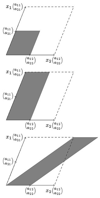
Geometric interpretation of Cramer's rule. The areas of the second and third shaded parallelograms are the same and the second is x 1 {\displaystyle x_{1}} times the first. From this equality Cramer's rule follows. source ↗

Cramer's rule has a geometric interpretation that can be considered also a proof or simply giving insight about its geometric nature. These geometric arguments work in general and not only in the case of two equations with two unknowns presented here.

Given the system of equations

a 11 x 1 + a 12 x 2 = b 1 a 21 x 1 + a 22 x 2 = b 2 {\displaystyle {\begin{matrix}a_{11}x_{1}+a_{12}x_{2}&=b_{1}\\a_{21}x_{1}+a_{22}x_{2}&=b_{2}\end{matrix}}}

it can be considered as an equation between vectors

x 1 ( a 11 a 21 ) + x 2 ( a 12 a 22 ) = ( b 1 b 2 ) . {\displaystyle x_{1}{\binom {a_{11}}{a_{21}}}+x_{2}{\binom {a_{12}}{a_{22}}}={\binom {b_{1}}{b_{2}}}.}

The area of the parallelogram determined by ( a 11 a 21 ) {\displaystyle {\binom {a_{11}}{a_{21}}}} and ( a 12 a 22 ) {\displaystyle {\binom {a_{12}}{a_{22}}}} is given by the determinant of the system of equations:

| a 11 a 12 a 21 a 22 | . {\displaystyle {\begin{vmatrix}a_{11}&a_{12}\\a_{21}&a_{22}\end{vmatrix}}.}

In general, when there are more variables and equations, the determinant of n vectors of length n will give the volume of the parallelepiped determined by those vectors in the n-th dimensional Euclidean space.

Animated 3D illustration of Cramer's rule as a ratio of determinants source ↗

Therefore, the area of the parallelogram determined by x 1 ( a 11 a 21 ) {\displaystyle x_{1}{\binom {a_{11}}{a_{21}}}} and ( a 12 a 22 ) {\displaystyle {\binom {a_{12}}{a_{22}}}} has to be x 1 {\displaystyle x_{1}} times the area of the first one since one of the sides has been multiplied by this factor. Now, this last parallelogram, by Cavalieri's principle, has the same area as the parallelogram determined by ( b 1 b 2 ) = x 1 ( a 11 a 21 ) + x 2 ( a 12 a 22 ) {\displaystyle {\binom {b_{1}}{b_{2}}}=x_{1}{\binom {a_{11}}{a_{21}}}+x_{2}{\binom {a_{12}}{a_{22}}}} and ( a 12 a 22 ) . {\displaystyle {\binom {a_{12}}{a_{22}}}.}

Equating the areas of this last and the second parallelogram gives the equation

| b 1 a 12 b 2 a 22 | = | a 11 x 1 a 12 a 21 x 1 a 22 | = x 1 | a 11 a 12 a 21 a 22 | {\displaystyle {\begin{vmatrix}b_{1}&a_{12}\\b_{2}&a_{22}\end{vmatrix}}={\begin{vmatrix}a_{11}x_{1}&a_{12}\\a_{21}x_{1}&a_{22}\end{vmatrix}}=x_{1}{\begin{vmatrix}a_{11}&a_{12}\\a_{21}&a_{22}\end{vmatrix}}}

from which Cramer's rule follows.

Other proofs

A proof by abstract linear algebra

This is a restatement of the proof above in abstract language.

Consider the map x = ( x 1 , , x n ) 1 det A ( det ( A 1 ) , , det ( A n ) ) , {\displaystyle \mathbf {x} =(x_{1},\ldots ,x_{n})\mapsto {\frac {1}{\det A}}\left(\det(A_{1}),\ldots ,\det(A_{n})\right),} where A i {\displaystyle A_{i}} is the matrix A {\displaystyle A} with x {\displaystyle \mathbf {x} } substituted in the i {\displaystyle i} th column, as in Cramer's rule. Because of linearity of determinant in every column, this map is linear. Observe that it sends the i {\displaystyle i} th column of A {\displaystyle A} to the i {\displaystyle i} th basis vector e i = ( 0 , , 1 , , 0 ) {\displaystyle \mathbf {e} _{i}=(0,\ldots ,1,\ldots ,0)} (with 1 in the i {\displaystyle i} th place), because determinant of a matrix with a repeated column is 0. So we have a linear map which agrees with the inverse of A {\displaystyle A} on the column space; hence it agrees with A 1 {\displaystyle A^{-1}} on the span of the column space. Since A {\displaystyle A} is invertible, the column vectors span all of R n {\displaystyle \mathbb {R} ^{n}} , so our map really is the inverse of A {\displaystyle A} . Cramer's rule follows.

A short proof

A short proof of Cramer's rule 9 can be given by noticing that x 1 {\displaystyle x_{1}} is the determinant of the matrix

X 1 = [ x 1 0 0 0 x 2 1 0 0 x 3 0 1 0 x n 0 0 1 ] {\displaystyle X_{1}={\begin{bmatrix}x_{1}&0&0&\cdots &0\\x_{2}&1&0&\cdots &0\\x_{3}&0&1&\cdots &0\\\vdots &\vdots &\vdots &\ddots &\vdots \\x_{n}&0&0&\cdots &1\end{bmatrix}}}

On the other hand, assuming that our original matrix A is invertible, this matrix X 1 {\displaystyle X_{1}} has columns A 1 b , A 1 v 2 , , A 1 v n {\displaystyle A^{-1}\mathbf {b} ,A^{-1}\mathbf {v} _{2},\ldots ,A^{-1}\mathbf {v} _{n}} , where v n {\displaystyle \mathbf {v} _{n}} is the n-th column of the matrix A. Recall that the matrix A 1 {\displaystyle A_{1}} has columns b , v 2 , , v n {\displaystyle \mathbf {b} ,\mathbf {v} _{2},\ldots ,\mathbf {v} _{n}} , and therefore X 1 = A 1 A 1 {\displaystyle X_{1}=A^{-1}A_{1}} . Hence, by using that the determinant of the product of two matrices is the product of the determinants, we have

x 1 = det ( X 1 ) = det ( A 1 ) det ( A 1 ) = det ( A 1 ) det ( A ) . {\displaystyle x_{1}=\det(X_{1})=\det(A^{-1})\det(A_{1})={\frac {\det(A_{1})}{\det(A)}}.}

The proof for other x j {\displaystyle x_{j}} is similar.

Using Geometric Algebra

Inconsistent and indeterminate cases

A system of equations is said to be inconsistent when there are no solutions and it is called indeterminate when there is more than one solution. For linear equations, an indeterminate system will have infinitely many solutions (if it is over an infinite field), since the solutions can be expressed in terms of one or more parameters that can take arbitrary values.

Cramer's rule applies to the case where the coefficient determinant is nonzero. In the 2×2 case, if the coefficient determinant is zero, then the system is inconsistent if the numerator determinants are nonzero, or indeterminate if the numerator determinants are zero.

Example 1: An Indeterminate System

Consider the linear system

2 x y = 8 4 x 2 y = 16 {\displaystyle {\begin{matrix}2x-y&=8\\4x-2y&=16\end{matrix}}}

By inspection, the second equation is a multiple of the first, so there are infinitely many solutions. Applying Cramer's Rule gives

x = | 8 1 16 2 | | 2 1 4 2 | = 0 0 , y = | 2 8 4 16 | | 2 1 4 2 | = 0 0 {\displaystyle {\begin{aligned}x&={\frac {\begin{vmatrix}8&-1\\{16}&-2\end{vmatrix}}{\begin{vmatrix}2&-1\\4&-2\end{vmatrix}}}={0 \over 0},\quad y={\frac {\begin{vmatrix}2&8\\4&{16}\end{vmatrix}}{\begin{vmatrix}2&-1\\4&-2\end{vmatrix}}}={0 \over 0}\end{aligned}}}

which both have zero numerators and denominators, meaning the system has infinitely many solutions and is therefore indeterminate.

Example 2: An Inconsistent System

Consider the linear system

3 x 4 y = 1 3 x 4 y = 2 {\displaystyle {\begin{matrix}3x-4y&=1\\3x-4y&=2\end{matrix}}}

By inspection, the left hand side of both equations are identical, with different right hand sides. Therefore, the system is inconsistent, meaning there are no solutions. Applying Cramer's Rule gives

x = | 1 4 2 4 | | 3 4 3 4 | = 4 0 , y = | 3 1 3 2 | | 3 4 3 4 | = 3 0 {\displaystyle {\begin{aligned}x&={\frac {\begin{vmatrix}1&-4\\{2}&-4\end{vmatrix}}{\begin{vmatrix}3&-4\\3&-4\end{vmatrix}}}={4 \over 0},\quad y={\frac {\begin{vmatrix}3&1\\3&{2}\end{vmatrix}}{\begin{vmatrix}3&-4\\3&-4\end{vmatrix}}}={3 \over 0}\end{aligned}}}

which are both undefined due to division by zero, however the non-zero numerators means the system has no solutions and is therefore inconsistent.

For 3×3 or higher systems, the only thing one can say when the coefficient determinant equals zero is that if any of the numerator determinants are nonzero, then the system must be inconsistent. However, having all determinants zero does not imply that the system is indeterminate. A simple example where all determinants vanish (equal zero) but the system is still inconsistent is the 3×3 system x+y+z=1, x+y+z=2, x+y+z=3.

Practical Considerations

Cramer's rule, implemented in a naive way, is computationally inefficient for systems of more than two or three equations.10 In the case of n equations in n unknowns, it requires computation of n + 1 determinants, while Gaussian elimination produces the result with the same (up to a constant factor independent of n {\displaystyle n} ) computational complexity as the computation of a single determinant.1112 Moreover, the Bareiss algorithm is a simple modification of Gaussian elimination that produces in a single computation a matrix whose nonzero entries are the determinants involved in Cramer's rule. In 1983, an algorithm for solving the system using Cramer's rule in n 3 + O ( n 2 ) {\displaystyle n^{3}+O(n^{2})} operations was proposed13. This algorithm can use permutations exactly like those in the Gaussian method. Therefore, if approximate calculation methods are used, the solution will be more stable than the solution using the Gaussian method, since the first steps are calculated without error, before rounding off the numbers. In 1991, an algorithm with complexity of n 3 / 2 + O ( n 2 ) {\displaystyle n^{3}/2+O(n^{2})} operations was published. 14. In 1997, an algorithm for solving a system using Cramer's rule with complexity equal to that of matrix multiplication was proposed.15. For example, for the Strassen's Multiplication Algorithm, this algorithm computes the solution in ( 7 / 15 ) n log 2 ( 7 ) + O ( n 2 ) {\displaystyle (7/15)n^{\log _{2}(7)}+O(n^{2})} operations.

See also

See also

References

References

  1. Cramer, Gabriel (1750). "Introduction à l'Analyse des lignes Courbes algébriques" (in French). Geneva: Europeana. pp. 656–659. Retrieved 2012-05-18.
  2. Kosinski, A. A. (2001). "Cramer's Rule is due to Cramer". Mathematics Magazine. 74 (4): 310–312. doi:10.2307/2691101. JSTOR 2691101.
  3. MacLaurin, Colin (1748). A Treatise of Algebra, in Three Parts. Printed for A. Millar & J. Nourse.
  4. Boyer, Carl B. (1968). A History of Mathematics (2nd ed.). Wiley. p. 431.
  5. Katz, Victor (2004). A History of Mathematics (Brief ed.). Pearson Education. pp. 378–379.
  6. Hedman, Bruce A. (1999). "An Earlier Date for "Cramer's Rule"" (PDF). Historia Mathematica. 26 (4): 365–368. doi:10.1006/hmat.1999.2247. S2CID 121056843.
  7. Zhiming Gong; M. Aldeen; L. Elsner (2002). "A note on a generalized Cramer's rule". Linear Algebra and Its Applications. 340 (1–3): 253–254. doi:10.1016/S0024-3795(01)00469-4.
  8. Levi-Civita, Tullio (1926). The Absolute Differential Calculus (Calculus of Tensors). Dover. pp. 111–112. ISBN 9780486634012. {{cite book}}: ISBN / Date incompatibility (help)
  9. Robinson, Stephen M. (1970). "A Short Proof of Cramer's Rule". Mathematics Magazine. 43 (2): 94–95. doi:10.1080/0025570X.1970.11976018.
  10. David Poole (2014). Linear Algebra: A Modern Introduction. Cengage Learning. p. 276. ISBN 978-1-285-98283-0.
  11. Joe D. Hoffman; Steven Frankel (2001). Numerical Methods for Engineers and Scientists, Second Edition. CRC Press. p. 30. ISBN 978-0-8247-0443-8.
  12. Thomas S. Shores (2007). Applied Linear Algebra and Matrix Analysis. Springer Science & Business Media. p. 132. ISBN 978-0-387-48947-6.
  13. Malaschonok G. I. Solution of a system of linear equations in an integral domain, Zh. Vychisl. Mat. i Mat. Fiz. V.23, No. 6, 1983, 1497–1500, (Russian), https://www.mathnet.ru/php/archive.phtml?wshow=paper&jrnid=zvmmf&paperid=4484&option_lang=rus U.S.S.R. Comput. Math. Math. Phys., 23:6 (1983), 133–135. (Engl.transl.) https://doi.org/10.48550/arXiv.1711.09452
  14. Malaschonok G. I. Algorithms for the solution of systems of linear equations in commutative rings. Effective methods in Algebraic Geometry, Progr. Math., Vol. 94, Birkhauser Boston, Boston, MA, 1991, pp. 289–298. https://arxiv.org/abs/1711.11471
  15. Malashonok G. I. Recursive Method for the Solution of Systems of Linear Equations // Computational Mathematics / A. Sydow Ed. — Proceedings of the 15th IMACS World Congress, Vol. I. — Berlin: Wissenschaft & Technik Verlag, 1997. — P. 475–480. https://arxiv.org/abs/1703.10232
External links