Convex analysis

Convex analysis is the branch of mathematics that studies convex sets, convex functions, and their applications to optimization, functional analysis, variational analysis, convex geometry, economics, and related fields. A set is convex if it contains every line segment joining two of its points. A function is convex if its value at a weighted average of two points is no greater than the corresponding weighted average of its values. Informally, convex sets have no inward dents, and convex functions have graphs that bend upward.

Convexity implies certain global features of a problem. For example, in a convex optimization problem, every local minimum is also a global minimum. Convex sets can often be separated by hyperplanes, and convex functions can be studied through supporting affine functions. Convex analysis is a common thread in modern optimization, duality theory, and the study of nonsmooth problems. The tools of convex analysis include the epigraph of a function, the subdifferential, the Legendre–Fenchel transform, and the Fenchel–Moreau theorem. These allow many constrained problems to be rewritten in geometric form and many optimization problems to be paired with dual problems.

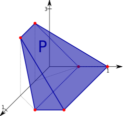
The simplest convex subsets of Euclidean space are points, line segments, affine subspaces, half-spaces, balls, cones, and convex polytopes. Intersections of convex sets are convex, so many complicated convex sets can be described as intersections of simpler ones. For example, a polyhedron in ${\displaystyle \mathbb {R} ^{n}}$ is the intersection of finitely many half-spaces.

Examples of convex functions include affine functions, quadratic functions (with positive semidefinite Hessian), norms, and the maximum of a family of affine functions. For instance,

${\displaystyle f(x)=x^{2}}$

is convex on the real line, and

${\displaystyle f(x)=\|x\|}$

is convex on any normed vector space.

Convex analysis also uses extended real-valued functions, which may take the value ${\displaystyle +\infty }$. This convention allows constraints to be incorporated directly into a function. If ${\displaystyle C}$ is a convex set, its indicator function in convex analysis is defined by

${\displaystyle \iota _{C}(x)={\begin{cases}0,&x\in C,\\+\infty ,&x\notin C.\end{cases}}}$

Minimizing ${\displaystyle f}$ over ${\displaystyle C}$ is then the same as minimizing ${\displaystyle f+\iota _{C}}$ over the whole space.¹

A subset ${\displaystyle C}$ of a real vector space is convex if, whenever ${\displaystyle x,y\in C}$ and ${\displaystyle 0\leq t\leq 1}$,

${\displaystyle tx+(1-t)y\in C.}$

This means that the line segment between ${\displaystyle x}$ and ${\displaystyle y}$ lies entirely in ${\displaystyle C}$.

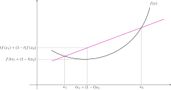
A function ${\displaystyle f:C\to \mathbb {R} }$, where ${\displaystyle C}$ is convex, is convex if

${\displaystyle f(tx+(1-t)y)\leq tf(x)+(1-t)f(y)}$

for all ${\displaystyle x,y\in C}$ and all ${\displaystyle 0\leq t\leq 1}$. It is strictly convex if the inequality is strict whenever ${\displaystyle x\neq y}$ and ${\displaystyle 0<t<1}$, apart from degenerate cases where the two sides are forced to be equal.

A function is convex if and only if its epigraph,

${\displaystyle \operatorname {epi} f=\{(x,r):f(x)\leq r\},}$

is a convex set. The epigraph is the region lying on or above the graph of the function. This observation is one reason convex functions and convex sets are studied together: statements about convex functions can often be translated into statements about convex sets in one higher dimension.¹²

For extended-real-valued functions ${\displaystyle f:X\to (-\infty ,+\infty ]}$, the effective domain is

${\displaystyle \operatorname {dom} f=\{x\in X:f(x)<+\infty \}.}$

A function is called proper if its effective domain is nonempty and it never takes the value ${\displaystyle -\infty }$. Proper convex functions are the usual objects of study in convex analysis.¹

Convex analysis takes different forms in finite-dimensional and infinite-dimensional spaces. In finite-dimensional Euclidean space, many geometric and topological complications are absent: all norms are equivalent, every linear functional is continuous, and closed and bounded sets are compact. As a result, many results can be stated using ordinary Euclidean topology. For example, a continuous convex function on a closed bounded convex subset of ${\displaystyle \mathbb {R} ^{n}}$ attains its minimum, and separation theorems can often be formulated in elementary geometric terms.¹³

In infinite-dimensional spaces, the topology of the underlying vector space becomes part of the theory. The relevant dual space is usually the continuous dual space, and many statements depend on whether one uses the norm topology, a weak topology, or another locally convex topology. Closed and bounded sets need not be compact, linear functionals may fail to be continuous unless continuity is assumed, and convex sets that are large in an algebraic sense may have empty interior in the norm topology.⁴⁵

These differences affect optimization. In finite dimensions, coercivity or compactness hypotheses often ensure the existence of minimizers. In infinite-dimensional spaces, minimizing sequences may fail to have convergent subsequences in the norm topology. Existence results therefore often use weak compactness, lower semicontinuity, and reflexivity assumptions, such as those in the direct methods in the calculus of variations. For example, in a reflexive Banach space, closed bounded convex sets have useful weak compactness properties, making weak lower semicontinuity a standard tool in variational problems.⁴⁶

Interior-point conditions also become more delicate in infinite dimensions. In finite-dimensional convex optimization, conditions such as Slater's condition are often expressed using the ordinary interior or relative interior of a convex set. In infinite-dimensional spaces, many natural convex sets have empty interior, so alternative notions such as algebraic interior, core, quasi-relative interior, or other constraint qualifications may be used.⁵

Duality is similarly affected. The Fenchel–Moreau theorem and related duality theorems require appropriate lower semicontinuity and convexity hypotheses relative to the chosen topology. Thus is closely tied to functional analysis, locally convex spaces, Banach spaces, Hilbert spaces, and monotone operator theory.¹²⁶

Convex analysis allows many problems to be formulated both in terms of the original vector space and its dual space. For example, a convex set can be described both in terms of its set of points and the set of hyperplanes that meet it. A non-empty closed convex set can also be described by its set of supporting hyperplanes.

For convex functions, duality also plays an important role. Given a proper convex function ${\displaystyle f:X\to \mathbb {R} }$, the supporting hyperplanes of the epigraph are encoded by the convex conjugate, defined at a point ${\displaystyle x^{*}\in X^{*}}$ by⁷ $${\displaystyle f^{*}(x^{*})=\sup _{z\in X}\left\{\left\langle x^{*},z\right\rangle -f(z)\right\}}$$ where the brackets ${\displaystyle \left\langle \cdot ,\cdot \right\rangle }$ denote the canonical duality ${\displaystyle \left\langle x^{*},z\right\rangle :=x^{*}(z).}$ The function ${\displaystyle f^{*}(x^{*})}$ makes sense, more generally, regardless of the convexity of ${\displaystyle f}$, but the convex conjugate of any function is always convex.

Geometrically, the convex conjugate describes the supporting affine functions of the epigraph of ${\displaystyle f}$. For a fixed dual vector ${\displaystyle x^{*}}$, the value ${\displaystyle f^{*}(x^{*})}$ is the smallest constant ${\displaystyle c}$ such that the affine function

${\displaystyle x\mapsto \langle x^{*},x\rangle -c}$

lies below ${\displaystyle f}$ on its domain. Indeed, the definition of the conjugate is equivalent to

${\displaystyle \langle x^{*},x\rangle -f^{*}(x^{*})\leq f(x)}$

for all ${\displaystyle x}$. Hence the hyperplane

${\displaystyle r=\langle x^{*},x\rangle -f^{*}(x^{*})}$

lies below the epigraph of ${\displaystyle f}$. If this hyperplane touches the epigraph at ${\displaystyle (x,f(x))}$, then it is a supporting hyperplane there. This touching condition is equivalent to

${\displaystyle f(x)+f^{*}(x^{*})=\langle x^{*},x\rangle ,}$

or equivalently ${\displaystyle x^{*}\in \partial f(x)}$, the subdifferential of ${\displaystyle f}$ at ${\displaystyle x}$.

Many problems in convex analysis have a corresponding dual problem. In general, the dual problem is formulated on a dual vector space and gives bounds on the value of the original, or primal, problem. Under additional hypotheses these bounds are exact, a property known as strong duality.

A simple geometric example is the relation between a norm and its dual norm. If ${\displaystyle \|\cdot \|}$ is a norm on ${\displaystyle X}$, its dual norm on ${\displaystyle X^{*}}$ is defined by

${\displaystyle \|x^{*}\|_{*}=\sup _{\|x\|\leq 1}\langle x^{*},x\rangle .}$

Equivalently, the norm of ${\displaystyle x}$ can be recovered from the dual unit ball:

${\displaystyle \|x\|=\sup _{\|x^{*}\|_{*}\leq 1}\langle x^{*},x\rangle .}$

Thus the unit ball of a norm and the unit ball of the dual norm determine one another by polar duality. More generally, if ${\displaystyle C}$ is a convex set containing the origin, its polar set is

${\displaystyle C^{\circ }=\{x^{*}\in X^{*}:\langle x^{*},x\rangle \leq 1{\text{ for all }}x\in C\}.}$

Under suitable closedness hypotheses, the bipolar theorem says that ${\displaystyle C}$ can be recovered from its polar by taking the polar again.¹

A central analytic example is Fenchel duality. Let ${\displaystyle A:X\to Y}$ be a continuous linear map between locally convex spaces, and let ${\displaystyle f:X\to (-\infty ,+\infty ]}$ and ${\displaystyle g:Y\to (-\infty ,+\infty ]}$ be proper convex functions. The primal problem

${\displaystyle \inf _{x\in X}\{f(x)+g(Ax)\}}$

has the Fenchel dual problem

${\displaystyle \sup _{y^{*}\in Y^{*}}\{-f^{*}(-A^{*}y^{*})-g^{*}(y^{*})\},}$

where ${\displaystyle A^{*}:Y^{*}\to X^{*}}$ is the adjoint map. The inequality

${\displaystyle \sup _{y^{*}\in Y^{*}}\{-f^{*}(-A^{*}y^{*})-g^{*}(y^{*})\}\leq \inf _{x\in X}\{f(x)+g(Ax)\}}$

is an instance of weak duality. Under standard regularity or constraint qualification assumptions, equality holds.¹⁸

The usual Lagrange duality of constrained optimization is a special case of this general principle. For a convex optimization problem

${\displaystyle \min _{x}f_{0}(x)\quad {\text{subject to}}\quad f_{i}(x)\leq 0,\quad i=1,\ldots ,m,}$

where the functions ${\displaystyle f_{i}}$ are convex, the Lagrangian is

${\displaystyle L(x,\lambda )=f_{0}(x)+\sum _{i=1}^{m}\lambda _{i}f_{i}(x),\qquad \lambda _{i}\geq 0.}$

The associated dual function is

${\displaystyle q(\lambda )=\inf _{x}L(x,\lambda ),}$

and the Lagrange dual problem is

${\displaystyle \sup _{\lambda \geq 0}q(\lambda ).}$

Every feasible choice of the multiplier vector ${\displaystyle \lambda }$ gives a lower bound on the primal minimum. When a condition such as Slater's condition holds, the optimal dual value equals the optimal primal value for many finite-dimensional convex programs.⁹

For example, the linear programming problem

${\displaystyle \min\{c^{T}x:Ax=b,\ x\geq 0\}}$

has the dual problem

${\displaystyle \max\{b^{T}y:A^{T}y\leq c\}.}$

The dual variables ${\displaystyle y}$ may be interpreted as the multipliers attached to the equality constraints ${\displaystyle Ax=b}$.

Duality is especially useful for certifying solutions to optimization problems. If a feasible primal point and a feasible dual point have the same objective value, then both are optimal. In this way, convex duality converts an optimization problem into a pair of mutually checking problems, one in the original space and one in the dual space.

A general way to construct dual problems in convex analysis uses a perturbation function. Let ${\displaystyle X}$ and ${\displaystyle Y}$ be locally convex spaces, and let

${\displaystyle F:X\times Y\to (-\infty ,+\infty ]}$

be a proper convex function. The associated value function is

${\displaystyle p(y)=\inf _{x\in X}F(x,y).}$

The original, or primal, problem is the computation of ${\displaystyle p(0)}$, that is,

${\displaystyle \inf _{x\in X}F(x,0).}$

The convex conjugate of ${\displaystyle F}$ is defined on ${\displaystyle X^{*}\times Y^{*}}$. Since

${\displaystyle p^{*}(y^{*})=F^{*}(0,y^{*}),}$

the biconjugate inequality ${\displaystyle p^{**}(0)\leq p(0)}$ gives the dual problem

${\displaystyle \sup _{y^{*}\in Y^{*}}-F^{*}(0,y^{*}).}$

Thus weak duality takes the form

${\displaystyle \sup _{y^{*}\in Y^{*}}-F^{*}(0,y^{*})\leq \inf _{x\in X}F(x,0).}$

When equality holds, the primal and dual problems are said to satisfy strong duality. Conditions ensuring equality are usually stated as regularity or constraint-qualification hypotheses, such as interior-point conditions in finite-dimensional convex optimization.¹⁸

This perturbation framework includes many familiar dualities as special cases, including Fenchel duality and Lagrange duality. Different choices of the perturbation function ${\displaystyle F}$ can lead to different dual problems for the same primal optimization problem.

Convex functions need not be differentiable. For example, the absolute value function ${\displaystyle f(x)=|x|}$ is convex but is not differentiable at ${\displaystyle x=0}$. Convex analysis therefore uses a generalized derivative called a subgradient.

Let ${\displaystyle f:X\to (-\infty ,+\infty ]}$ be a convex function on a real vector space, and let ${\displaystyle X^{*}}$ be a suitable dual space. A functional ${\displaystyle x^{*}\in X^{*}}$ is a subgradient of ${\displaystyle f}$ at ${\displaystyle x}$ if

${\displaystyle f(z)\geq f(x)+\langle x^{*},z-x\rangle }$

for all ${\displaystyle z\in X}$. The set of all subgradients at ${\displaystyle x}$ is the subdifferential of ${\displaystyle f}$ at ${\displaystyle x}$, denoted ${\displaystyle \partial f(x)}$.¹³

Geometrically, a subgradient defines a supporting hyperplane to the epigraph of ${\displaystyle f}$. If ${\displaystyle f}$ is differentiable at ${\displaystyle x}$, then the subdifferential consists of the ordinary derivative. In finite-dimensional Euclidean space this is written

${\displaystyle \partial f(x)=\{\nabla f(x)\}.}$

Subgradients give a basic optimality condition. A point ${\displaystyle x}$ minimizes a proper convex function ${\displaystyle f}$ if and only if

${\displaystyle 0\in \partial f(x).}$

This generalizes the familiar condition ${\displaystyle \nabla f(x)=0}$ for differentiable functions.

Convex analysis often studies functions that are lower semi-continuous rather than continuous. A function ${\displaystyle f:X\to (-\infty ,+\infty ]}$ is lower semicontinuous if, roughly speaking, its values cannot suddenly jump downward. Equivalently, in a topological vector space, ${\displaystyle f}$ is lower semicontinuous if the sublevel sets

${\displaystyle \{x\in X:f(x)\leq a\}}$

are closed for all real numbers ${\displaystyle a}$. For convex functions, lower semicontinuity is also equivalent to closedness of the epigraph:

${\displaystyle \operatorname {epi} f=\{(x,r):f(x)\leq r\}.}$

Thus lower semicontinuous convex functions are often called closed convex functions.¹²

Lower semicontinuity is important in optimization because it helps ensure that minimizing limits do not lose the value of the function. If a sequence or net ${\displaystyle x_{i}}$ converges to ${\displaystyle x}$, lower semicontinuity gives

${\displaystyle f(x)\leq \liminf _{i}f(x_{i}).}$

This condition is weaker than continuity, but it is often strong enough for existence theorems, especially when combined with compactness or weak compactness assumptions.⁴⁶

The condition also appears in duality. The convex conjugate of any function is convex and lower semicontinuous with respect to the appropriate weak-* topology. The conjugate of the conjugate, or biconjugate, gives the closed convex envelope of the original function. In one common form, the Fenchel–Moreau theorem states that a proper function on a locally convex space satisfies

${\displaystyle f=f^{**}}$

if and only if ${\displaystyle f}$ is convex and lower semicontinuous. Equivalently, closed proper convex functions are exactly the functions that can be recovered from their affine minorants.¹⁷

In convex optimization, the objective is to minimize a convex function over a convex set. Convexity ensures that every local minimum is a global minimum, and duality often provides certificates of optimality. Linear programming, quadratic programming, semidefinite programming, and many methods in statistics and machine learning use this framework.⁹

Convex analysis is also connected with convex geometry, which studies convex bodies, polytopes, supporting hyperplanes, mixed volumes, and related geometric inequalities. Classical finite-dimensional results such as Carathéodory's theorem (convex hull), Helly's theorem, and Radon's theorem describe the combinatorial and geometric structure of convex hulls. These theorems are usually regarded as part of convex geometry, but they provide much of the geometric background for convex analysis.¹

In functional analysis, compact convex sets are studied through their extreme points. The Krein–Milman theorem states that, under suitable hypotheses, a compact convex set in a locally convex space is generated by its extreme points. Choquet theory refines this idea by representing points of compact convex sets as barycenters of probability measures supported on extreme points. This can be viewed as an infinite-dimensional analogue of writing a point of a polytope as a convex combination of its vertices.¹⁰¹¹

Convexity is also used in probability theory. Jensen's inequality compares the value of a convex function at an average with the average of its values. Convex order compares probability measures by testing them against convex functions, and large deviations theory uses the Legendre–Fenchel transform to express rate functions as convex conjugates of logarithmic moment generating functions.¹²

In optimal transport, the Kantorovich formulation of the transport problem is a convex optimization problem over probability measures, and Kantorovich duality is a form of convex duality. For the quadratic cost on Euclidean space, Brenier's theorem relates optimal transport maps to gradients of convex functions, connecting optimal transport with the Monge–Ampère equation.¹³¹⁴

Several areas use modified notions of convexity adapted to different structures. In the calculus of variations, rank-one convexity, polyconvexity, and quasiconvexity arise in vector-valued variational problems. In metric geometry and optimization on manifolds, geodesic convexity replaces line segments by geodesics. In several complex variables, notions such as pseudoconvexity, holomorphic convexity, polynomial convexity, and plurisubharmonic functions play roles analogous in some respects to convexity in real analysis.¹⁵¹⁶¹⁷

See also

See also

• Convexity in economics – Significant topic in economics
  • Non-convexity (economics) – Violations of the convexity assumptions of elementary economics
• List of convexity topics
• Werner Fenchel – German mathematician (1905–1988)

Notes

Notes

1. Rockafellar 1970.
2. Rockafellar & Wets 2009.
3. Hiriart-Urruty & Lemaréchal 2001.
4. Rudin 1991.
5. Zălinescu 2002.
6. Bauschke & Combettes 2017.
7. Zălinescu 2002, pp. 75–79.
8. Zălinescu 2002, pp. 106–113.
9. Boyd & Vandenberghe 2004.
10. Phelps 2001.
11. Alfsen 1971.
12. Dembo & Zeitouni 1998.
13. Villani 2003.
14. Villani 2009.
15. Dacorogna 2008.
16. Bridson & Haefliger 1999.
17. Hörmander 1994.

References

References

• Alfsen, Erik M. (1971). Compact Convex Sets and Boundary Integrals. Springer. ISBN 978-3-642-65011-6.
• Bridson, Martin R.; Haefliger, André (1999). Metric Spaces of Non-Positive Curvature. Springer. ISBN 978-3-540-64324-1.
• Dacorogna, Bernard (2008). Direct Methods in the Calculus of Variations (2 ed.). Springer. ISBN 978-0-387-35779-9.
• Dembo, Amir; Zeitouni, Ofer (1998). Large Deviations Techniques and Applications (2 ed.). Springer. ISBN 978-0-387-98406-3.
• Hörmander, Lars (1994). Notions of Convexity. Birkhäuser.
• Phelps, Robert R. (2001). Lectures on Choquet's Theorem (2 ed.). Springer. ISBN 978-3-540-41834-4.
• Villani, Cédric (2003). Topics in Optimal Transportation. American Mathematical Society. ISBN 978-0-8218-3312-4.
• Villani, Cédric (2009). Optimal Transport: Old and New. Springer. ISBN 978-3-540-71049-3.
• Borwein, Jonathan; Lewis, Adrian (2006), Convex Analysis and Nonlinear Optimization: Theory and Examples (2 ed.), Springer, ISBN 978-0-387-29570-1.
• Boţ, Radu Ioan; Wanka, Gert; Grad, Sorin-Mihai (2009), Duality in Vector Optimization, Springer, ISBN 978-3-642-02885-4.
• Csetnek, Ernö Robert (2010), Overcoming the failure of the classical generalized interior-point regularity conditions in convex optimization. Applications of the duality theory to enlargements of maximal monotone operators, Logos Verlag Berlin GmbH, ISBN 978-3-8325-2503-3.
• Rockafellar, R. Tyrrell (1997) [1970], Convex Analysis, Princeton, NJ: Princeton University Press, ISBN 978-0-691-01586-6.
• Bauschke, Heinz H.; Combettes, Patrick L. (28 February 2017). Convex Analysis and Monotone Operator Theory in Hilbert Spaces. CMS Books in Mathematics. Springer Science & Business Media. ISBN 978-3-319-48311-5. OCLC 1037059594.
• Boyd, Stephen; Vandenberghe, Lieven (8 March 2004). Convex Optimization. Cambridge Series in Statistical and Probabilistic Mathematics. Cambridge, U.K. New York: Cambridge University Press. ISBN 978-0-521-83378-3. OCLC 53331084.
• Hiriart-Urruty, J.-B.; Lemaréchal, C. (2001). Fundamentals of convex analysis. Berlin: Springer-Verlag. ISBN 978-3-540-42205-1.
• Kusraev, A.G.; Kutateladze, Semen Samsonovich (1995). Subdifferentials: Theory and Applications. Dordrecht: Kluwer Academic Publishers. ISBN 978-94-011-0265-0.
• Rockafellar, R. Tyrrell; Wets, Roger J.-B. (26 June 2009). Variational Analysis. Grundlehren der mathematischen Wissenschaften. Vol. 317. Berlin New York: Springer Science & Business Media. ISBN 9783642024313. OCLC 883392544.
• Rockafellar, R. Tyrrell (1970). Convex analysis. Princeton mathematical series. Princeton, N.J: Princeton University Press. ISBN 978-0-691-08069-7.
• Rudin, Walter (1991). Functional Analysis. International Series in Pure and Applied Mathematics. Vol. 8 (Second ed.). New York, NY: McGraw-Hill Science/Engineering/Math. ISBN 978-0-07-054236-5. OCLC 21163277.
• Singer, Ivan (1997). Abstract convex analysis. Canadian Mathematical Society series of monographs and advanced texts. New York: John Wiley & Sons, Inc. pp. xxii+491. ISBN 0-471-16015-6. MR 1461544.
• Stoer, J.; Witzgall, C. (1970). Convexity and optimization in finite dimensions. Vol. 1. Berlin: Springer. ISBN 978-0-387-04835-2.
• Zălinescu, Constantin (30 July 2002). Convex Analysis in General Vector Spaces. River Edge, N.J. London: World Scientific Publishing. ISBN 978-981-4488-15-0. MR 1921556. OCLC 285163112 – via Internet Archive.

External links

External links

• Media related to Convex analysis at Wikimedia Commons