Change of basis

A linear combination of one basis of vectors (purple) yields new vectors (red). If these are linearly independent, they form a new basis. The linear combinations relating the initial basis to the other extend to a linear transformation, called the change of basis.

A vector represented by two different bases (purple and red arrows).

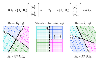
In mathematics, an ordered basis of a vector space of finite dimension n allows representing uniquely any element of the vector space by a coordinate vector, which is a finite sequence of n scalars called coordinates. If two different bases are considered, the coordinate vector that represents a vector v on one basis is, in general, different from the coordinate vector that represents v on the other basis. A change of basis consists of converting every assertion expressed in terms of coordinates relative to one basis into an assertion expressed in terms of coordinates relative to the other basis.¹²³

Such a conversion results from the change-of-basis formula, which expresses the coordinates relative to one basis in terms of the coordinates relative to the other basis. Using matrices, this formula can be written

${\displaystyle \mathbf {x} _{\mathrm {old} }=A~\mathbf {x} _{\mathrm {new} },}$

where ${\displaystyle \mathbf {x} _{\mathrm {old} }}$ and ${\displaystyle \mathbf {x} _{\mathrm {new} }}$ are the column vectors of the coordinates of the same vector on the "old" (initially defined) and "new" (other) bases. ${\displaystyle A}$ is the change-of-basis matrix (also called transition matrix), which is the matrix whose columns are the coordinates of the "new" basis vectors on the "old" basis.

A change of basis is sometimes called a change of coordinates, although it excludes many coordinate transformations. For applications in physics and specially in mechanics, a change of basis often involves the transformation of an orthonormal basis, understood as a rotation in physical space, thus excluding translations.

This article deals mainly with finite-dimensional vector spaces. However, many of the presented principles are also valid for infinite-dimensional vector spaces.

Let ${\displaystyle B_{\mathrm {old} }=(v_{1},\ldots ,v_{n})}$ be a basis of a finite-dimensional vector space V over a field F.^b

For j = 1, ..., n, one can define a vector w_j by its coordinates ${\displaystyle a_{i,j}}$ over ${\displaystyle B_{\mathrm {old} }\colon }$

${\displaystyle w_{j}=\sum _{i=1}^{n}a_{i,j}v_{i}.}$

Let

${\displaystyle A=\left(a_{i,j}\right)_{i,j}}$

be the matrix whose j-th column is formed by the coordinates of w_j. (Here and in what follows, the index i refers always to the rows of A and the ${\displaystyle v_{i},}$ while the index j refers always to the columns of A and the ${\displaystyle w_{j};}$ such a convention is useful for avoiding errors in explicit computations.)

Setting ${\displaystyle B_{\mathrm {new} }=(w_{1},\ldots ,w_{n}),}$ one has that ${\displaystyle B_{\mathrm {new} }}$ is a basis of V if and only if the matrix A is invertible, or equivalently, if it has a nonzero determinant. In this case, A is said to be the change-of-basis matrix from the basis ${\displaystyle B_{\mathrm {old} }}$ to the basis ${\displaystyle B_{\mathrm {new} }.}$

Given a vector ${\displaystyle u\in V,}$ let ${\displaystyle (x_{1},\ldots ,x_{n})}$ be the coordinates of ${\displaystyle u}$ over ${\displaystyle B_{\mathrm {old} },}$ and ${\displaystyle (y_{1},\ldots ,y_{n})}$ its coordinates over ${\displaystyle B_{\mathrm {new} };}$ that is

${\displaystyle u=\sum _{i=1}^{n}x_{i}v_{i}=\sum _{j=1}^{n}y_{j}w_{j}.}$

(One could take the same summation index for the two sums, but choosing systematically the indexes i for the old basis and j for the new one makes clearer the formulas that follows, and helps avoiding errors in proofs and explicit computations.)

The change-of-basis formula expresses the coordinates over the old basis in terms of the coordinates over the new basis. With above notation, it is

${\displaystyle x_{i}=\sum _{j=1}^{n}a_{i,j}y_{j}\qquad {\text{for }}i=1,\ldots ,n.}$

In terms of matrices, the change-of-basis formula is

${\displaystyle \mathbf {x} =A~\mathbf {y} ,}$

where ${\displaystyle \mathbf {x} }$ and ${\displaystyle \mathbf {y} }$ are the column vectors of the coordinates of ${\displaystyle u}$ over ${\displaystyle B_{\mathrm {old} }}$ and ${\displaystyle B_{\mathrm {new} },}$ respectively. (This reverse terminology is confusing, but internationally adopted.)

Proof: Using the above definition of the change-of-basis matrix, one has

${\displaystyle {\begin{aligned}u&=\sum _{j=1}^{n}y_{j}w_{j}\\&=\sum _{j=1}^{n}\left(y_{j}\sum _{i=1}^{n}a_{i,j}v_{i}\right)\\&=\sum _{i=1}^{n}\left(\sum _{j=1}^{n}a_{i,j}y_{j}\right)v_{i}.\end{aligned}}}$

As ${\displaystyle u=\textstyle \sum _{i=1}^{n}x_{i}v_{i},}$ the change-of-basis formula results from the uniqueness of the decomposition of a vector over a basis.

Consider the Euclidean vector space ${\displaystyle \mathbb {R} ^{2}}$ and its standard basis, consisting of the vectors ${\displaystyle v_{1}}$ and ${\displaystyle v_{2}}$ with column vectors

${\displaystyle \mathbf {v_{1}} ={\begin{bmatrix}1\\0\end{bmatrix}}\quad }$ and ${\displaystyle \quad \mathbf {v_{2}} ={\begin{bmatrix}0\\1\end{bmatrix}}.}$

Rotating them by an angle of ${\displaystyle t}$ gives a "new" basis, formed by the vectors ${\displaystyle w_{1}}$ and ${\displaystyle w_{2}}$ with column vectors

${\displaystyle \mathbf {w_{1}} ={\begin{bmatrix}\cos t\\\sin t\end{bmatrix}}\quad }$ and ${\displaystyle \quad \mathbf {w_{2}} ={\begin{bmatrix}-\sin t\\\cos t\end{bmatrix}}.}$

So, the change-of-basis matrix is

${\displaystyle {\begin{bmatrix}\cos t&-\sin t\\\sin t&\cos t\end{bmatrix}}.}$

The change-of-basis formula asserts that, for a vector with "old" coordinates ${\displaystyle (x_{1},x_{2})}$ and "new" coordinates ${\displaystyle (y_{1},y_{2}),}$ one has

${\displaystyle {\begin{bmatrix}x_{1}\\x_{2}\end{bmatrix}}={\begin{bmatrix}\cos t&-\sin t\\\sin t&\cos t\end{bmatrix}}~{\begin{bmatrix}y_{1}\\y_{2}\end{bmatrix}}.}$

That is,

${\displaystyle {\begin{cases}x_{1}=y_{1}\cos t-y_{2}\sin t\\x_{2}=y_{1}\sin t+y_{2}\cos t.\end{cases}}}$

This may be shown by writing

${\displaystyle {\begin{aligned}y_{1}w_{1}+y_{2}w_{2}&=y_{1}{\Big (}(\cos t)~v_{1}+(\sin t)~v_{2}{\Big )}+y_{2}{\Big (}\!-(\sin t)~v_{1}+(\cos t)~v_{2}{\Big )}\\&={\big (}y_{1}\cos t-y_{2}\sin t{\big )}v_{1}+{\big (}y_{1}\sin t+y_{2}\cos t{\big )}v_{2}\\&=x_{1}v_{1}+x_{2}v_{2}.\end{aligned}}}$

Usually, a matrix represents a linear map, and the product of a matrix and a column vector represents the function application of the corresponding linear map to the vector whose coordinates form the column vector. The change-of-basis formula is a specific case of this general principle, although this is not immediately clear from its definition and proof.

When one says that a matrix represents a linear map, one refers implicitly to bases of implied vector spaces, and to the fact that the choice of a basis induces a linear isomorphism between a vector space and ${\displaystyle F^{n}}$, where F is the ground field of scalars. When only one basis is considered for each vector space, it is convenient to leave this isomorphism implicit, and to work up to an isomorphism. As several bases of the same vector space are considered here, a more accurate wording is required.

Let F be a field, the set ${\displaystyle F^{n}}$ of the n-tuples is an F-vector space whose addition and scalar multiplication are defined component-wise. Its standard basis is the basis that has as its i-th element the tuple with all components equal to 0 except the i-th one, equal to 1.

A basis ${\displaystyle B=(v_{1},\ldots ,v_{n})}$ of an F-vector space V defines a linear isomorphism ${\displaystyle \varphi \colon F^{n}\to V}$ by

${\displaystyle \varphi (x_{1},\ldots ,x_{n})=\sum _{i=1}^{n}x_{i}v_{i}.}$

Conversely, such a linear isomorphism defines a basis, which is the image by ${\displaystyle \varphi }$ of the standard basis of ${\displaystyle F^{n}.}$

Let ${\displaystyle B_{\mathrm {old} }=(v_{1},\ldots ,v_{n})}$ be the "old" basis of a change of basis, and ${\displaystyle \varphi _{\mathrm {old} }}$ the associated isomorphism. Given a change-of-basis (invertible) matrix A, one could consider it the matrix of an automorphism (a bijective endomorphism) ${\displaystyle \psi _{A}}$ of ${\displaystyle F^{n}.}$ Finally, define

${\displaystyle \varphi _{\mathrm {new} }=\varphi _{\mathrm {old} }\circ \psi _{A}}$

(where ${\displaystyle \circ }$ denotes function composition), and

${\displaystyle B_{\mathrm {new} }=\varphi _{\mathrm {new} }\left(\varphi _{\mathrm {old} }^{-1}(B_{\mathrm {old} })\right).}$

A straightforward verification shows that this definition of ${\displaystyle B_{\mathrm {new} }}$ is the same as that in the preceding section.

Now, by composing the equation ${\displaystyle \varphi _{\mathrm {new} }=\varphi _{\mathrm {old} }\circ \psi _{A}}$ with ${\displaystyle \varphi _{\mathrm {old} }^{-1}}$ on the left and ${\displaystyle \varphi _{\mathrm {new} }^{-1}}$ on the right, one gets

${\displaystyle \varphi _{\mathrm {old} }^{-1}=\psi _{A}\circ \varphi _{\mathrm {new} }^{-1}.}$

It follows that, for ${\displaystyle v\in V,}$ one has

${\displaystyle \varphi _{\mathrm {old} }^{-1}(v)=\psi _{A}\left(\varphi _{\mathrm {new} }^{-1}(v)\right),}$

which is the change-of-basis formula expressed in terms of linear maps instead of coordinates.

A function that has a vector space as its domain is commonly specified as a multivariate function whose variables are the coordinates on some basis of the vector on which the function is applied.

When the basis is changed, the expression of the function is changed. This change can be computed by substituting the "old" coordinates for their expressions in terms of the "new" coordinates. More precisely, if f(x) is the expression of the function in terms of the "old" coordinates, and if x = Ay is the change-of-basis formula, then f(Ay) is the expression of the same function in terms of the "new" coordinates.

The fact that the change-of-basis formula expresses the "old" coordinates in terms of the "new" ones may seem unnatural, but appears as useful, because no matrix inversion is needed here.

As the change-of-basis formula involves only linear functions, many function properties are kept by a change of basis. This allows defining these properties as properties of functions of a variable vector that are not related to any specific basis. So, a function whose domain is a vector space or a subset of it is

• a linear function,
• a polynomial function,
• a continuous function,
• a differentiable function,
• a smooth function,
• an analytic function,

if the multivariate function that represents it on some basis—and thus on every basis—has the same property.

This is specially useful in the theory of manifolds, as this allows extending the concepts of continuous, differentiable, smooth, and analytic functions to functions that are defined on a manifold.

Consider a linear map L: V → W from a vector space V of dimension n to a vector space W of dimension m. It is represented on "old" bases of V and W by an m×n matrix M. A change of basis is defined by an n×n change-of-basis matrix P for V, and an m×m change-of-basis matrix Q for W.

On the "new" bases, the matrix representation of L is

${\displaystyle M'=Q^{-1}MP.}$

This is a straightforward consequence of the change-of-basis formula.

Endomorphisms are linear maps from a vector space V to itself. For a change of basis, the formula of the preceding section applies, with the same change-of-basis matrix on both sides of the formula. That is, if M is the square matrix of an endomorphism of V on an "old" basis, and P is a change-of-basis matrix, then the matrix of the endomorphism on the "new" basis is

${\displaystyle M'=P^{-1}MP.}$

As every invertible matrix can be used as a change-of-basis matrix, this implies that two matrices are similar if and only if they represent the same endomorphism on two different bases.

A bilinear form on a vector space V over a field F is a function ${\displaystyle \varPhi \colon V\!\times V\to F}$ which is linear in both arguments. That is, ${\displaystyle \varPhi }$ is bilinear if the maps ${\displaystyle v\mapsto \varPhi (v,w)}$ and ${\displaystyle v\mapsto \varPhi (w,v)}$ are linear for every fixed ${\displaystyle w\in V.}$

The matrix ${\displaystyle \mathbf {\Phi } }$ of a bilinear form ${\displaystyle \varPhi }$ on a basis ${\displaystyle (v_{1},\ldots ,v_{n})}$ (the "old" basis) is the matrix whose entry of the i-th row and j-th column is ${\displaystyle \varPhi (v_{i},v_{j})}$. It follows that for two vectors v and w with coordinate column vectors v and w, one has

${\displaystyle \varPhi (v,w)=\mathbf {v} ^{\mathsf {T}}\mathbf {\Phi } \mathbf {w} ,}$

where ${\displaystyle \mathbf {v} ^{\mathsf {T}}}$ denotes the transpose of the column vector v.

For a change of basis with matrix P, a straightforward computation shows that the matrix of the bilinear form on the "new" basis is

${\displaystyle \mathbf {\Phi '} =P^{\mathsf {T}}\mathbf {\Phi } P.}$

A symmetric bilinear form is a bilinear form S such that ${\displaystyle S(v,w)=S(w,v)}$ for every v and w in V. It follows that the matrix of S on any basis is symmetric. This implies that the property of being a symmetric matrix must be kept by the above change-of-basis formula. One can also check this by noting that the transpose of a matrix product is the product of the transposes computed in the reverse order. Thus,

${\displaystyle (P^{\mathsf {T}}\mathbf {S} P)^{\mathsf {T}}=P^{\mathsf {T}}\mathbf {S} ^{\mathsf {T}}P;}$

finally, since the matrix S is symmetric,

${\displaystyle (P^{\mathsf {T}}\mathbf {S} P)^{\mathsf {T}}=P^{\mathsf {T}}\mathbf {S} P.}$

If the characteristic of the ground field F is not two, then for every symmetric bilinear form, there is a basis for which the matrix is diagonal. Moreover, the resulting nonzero entries on the diagonal are defined up to the multiplication by a square. So, if the ground field is the field ${\displaystyle \mathbb {R} }$ of the real numbers, these nonzero entries can be chosen to be either 1 or –1. Sylvester's law of inertia is a theorem that asserts that the numbers of 1 and of –1 depend only on the bilinear form, and not on the change of basis.

Symmetric bilinear forms over the reals are often encountered in geometry and physics, typically in the study of quadrics and of the inertia of a rigid body. In these cases, orthonormal bases are specially useful; this means that one generally prefers to restrict changes of basis to those that have an orthogonal change-of-basis matrix, that is, a matrix such that ${\displaystyle P^{\mathsf {T}}=P^{-1}.}$ Such matrices have the fundamental property that the change-of-basis formula is the same for a symmetric bilinear form and the endomorphism that is represented by the same symmetric matrix. The Spectral theorem asserts that, given such a symmetric matrix, there is an orthogonal change of basis such that the resulting matrix (of both the bilinear form and the endomorphism) is a diagonal matrix with the eigenvalues of the initial matrix on the diagonal. It follows that, over the reals, if the matrix of an endomorphism is symmetric, then it is diagonalizable.

References

- Anton (1987, pp. 221–237)
- Beauregard & Fraleigh (1973, pp. 240–243)
- Nering (1970, pp. 50–52)
- Anton, Howard (1987), Elementary Linear Algebra (5th ed.), New York: Wiley, ISBN 0-471-84819-0
- Beauregard, Raymond A.; Fraleigh, John B. (1973), A First Course In Linear Algebra: with Optional Introduction to Groups, Rings, and Fields, Boston: Houghton Mifflin Company, ISBN 0-395-14017-X
- Nering, Evar D. (1970), Linear Algebra and Matrix Theory (2nd ed.), New York: Wiley, LCCN 76091646
External links
- MIT Linear Algebra Lecture on Change of Basis, from MIT OpenCourseWare
- Khan Academy Lecture on Change of Basis, from Khan Academy