Article · Wikipedia archive · Last revised May 27, 2026

Bump function

In mathematical analysis, a bump function is a localized auxiliary function, usually chosen to be smooth and to have compact support. Bump functions are commonly used as cutoff functions, for example functions that are equal to 1 on a prescribed set and vanish outside a larger set, and as standard examples of kernels used to construct mollifiers.

Last revised
May 27, 2026
Read time
≈ 15 min
Length
3,447 w
Citations
11
Source
The graph of the bump function ( x , y ) R 2 Ψ ( r ) , {\displaystyle (x,y)\in \mathbb {R} ^{2}\mapsto \Psi (r),} where r = ( x 2 + y 2 ) 1 / 2 {\displaystyle r=\left(x^{2}+y^{2}\right)^{1/2}} and Ψ ( r ) = e 1 / ( 1 r 2 ) 1 { | r | < 1 } . {\displaystyle \Psi (r)=e^{-1/(1-r^{2})}\cdot \mathbf {1} _{\{|r|<1\}}.} source ↗

In mathematical analysis, a bump function is a localized auxiliary function, usually chosen to be smooth and to have compact support. Bump functions are commonly used as cutoff functions, for example functions that are equal to 1 on a prescribed set and vanish outside a larger set, and as standard examples of kernels used to construct mollifiers.

Some authors use the term more broadly for any compactly supported smooth function. Such functions are important examples of test functions, especially in distribution theory, but the terms "bump function" and "test function" are not synonymous in all contexts.

Examples
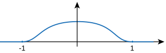
The 1d bump function Ψ ( x ) . {\displaystyle \Psi (x).} source ↗

The function Ψ : R R {\displaystyle \Psi :\mathbb {R} \to \mathbb {R} } given by Ψ ( x ) = { exp ( 1 x 2 1 ) ,  if  | x | < 1 , 0 ,  if  | x | 1 , {\displaystyle \Psi (x)={\begin{cases}\exp \left({\frac {1}{x^{2}-1}}\right),&{\text{ if }}|x|<1,\\0,&{\text{ if }}|x|\geq 1,\end{cases}}}

is an example of a bump function in one dimension. Note that the support of this function is the closed interval [ 1 , 1 ] {\displaystyle [-1,1]} . In fact, by definition of support, we have that supp ( Ψ ) := { x R : Ψ ( x ) 0 } ¯ = ( 1 , 1 ) ¯ {\displaystyle \operatorname {supp} (\Psi ):={\overline {\{x\in \mathbb {R} :\Psi (x)\neq 0\}}}={\overline {(-1,1)}}} , where the closure is taken with respect the Euclidean topology of the real line. The proof of smoothness follows along the same lines as for the related function discussed in the Non-analytic smooth function article. This function can be interpreted as the Gaussian function exp ( y 2 ) {\displaystyle \exp \left(-y^{2}\right)} scaled to fit into the unit disc: the substitution y 2 = 1 / ( 1 x 2 ) {\displaystyle y^{2}={1}/{\left(1-x^{2}\right)}} corresponds to sending x = ± 1 {\displaystyle x=\pm 1} to y = . {\displaystyle y=\infty .}

A simple example of a (square) bump function in n {\displaystyle n} variables is obtained by taking the product of n {\displaystyle n} copies of the above bump function in one variable, so Φ ( x 1 , x 2 , , x n ) = Ψ ( x 1 ) Ψ ( x 2 ) Ψ ( x n ) . {\displaystyle \Phi (x_{1},x_{2},\dots ,x_{n})=\Psi (x_{1})\Psi (x_{2})\cdots \Psi (x_{n}).}

A radially symmetric bump function in n {\displaystyle n} variables can be formed by taking the function Ψ n : R n R {\displaystyle \Psi _{n}:\mathbb {R} ^{n}\to \mathbb {R} } defined by Ψ n ( x ) = Ψ ( | x | ) {\displaystyle \Psi _{n}(\mathbf {x} )=\Psi (|\mathbf {x} |)} . This function is supported on the unit ball centered at the origin.

For another example, take an h {\displaystyle h} that is positive on ( c , d ) {\displaystyle (c,d)} and zero elsewhere, for example

h ( x ) = { exp ( 1 ( x c ) ( d x ) ) , c < x < d 0 , o t h e r w i s e {\displaystyle h(x)={\begin{cases}\exp \left(-{\frac {1}{(x-c)(d-x)}}\right),&c<x<d\\0,&\mathrm {otherwise} \end{cases}}} .


Smooth transition functions

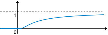
The non-analytic smooth function f(x) considered in the article. source ↗

A standard starting point is the function

f ( x ) = { e 1 x if  x > 0 , 0 if  x 0 , {\displaystyle f(x)={\begin{cases}e^{-{\frac {1}{x}}}&{\text{if }}x>0,\\0&{\text{if }}x\leq 0,\end{cases}}}

defined for every real number x.

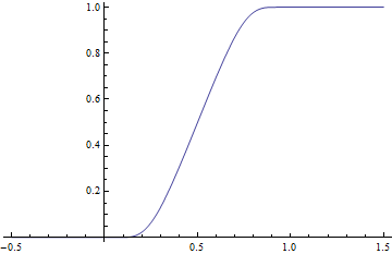
The smooth transition g from 0 to 1 defined here. source ↗

From this, define

g ( x ) = f ( x ) f ( x ) + f ( 1 x ) , x R . {\displaystyle g(x)={\frac {f(x)}{f(x)+f(1-x)}},\qquad x\in \mathbb {R} .}

The denominator is strictly positive everywhere on the real line, so g is smooth. Moreover, g(x) = 0 for x ≤ 0 and g(x) = 1 for x ≥ 1, so g gives a smooth transition from 0 to 1 on the unit interval [0, 1]. Rescaling gives a smooth transition on any interval [a, b] with a < b:

R x g ( x a b a ) . {\displaystyle \mathbb {R} \ni x\mapsto g{\Bigl (}{\frac {x-a}{b-a}}{\Bigr )}.}

A compactly supported bump function can be obtained by multiplying a rising transition by a falling transition. For real numbers a < bc < d, the function

R x g ( x a b a ) g ( d x d c ) {\displaystyle \mathbb {R} \ni x\mapsto g{\Bigl (}{\frac {x-a}{b-a}}{\Bigr )}\,g{\Bigl (}{\frac {d-x}{d-c}}{\Bigr )}}

is smooth, equals 1 on the closed interval [b, c], and vanishes outside the open interval (a, d). Thus it can serve as a bump function. When b < c the plateau has positive length; when b = c it degenerates to a single point, but the function is still smooth.

For example, taking a = 1 {\displaystyle a=-1} , b = c = 0 {\displaystyle b=c=0} , and d = 1 {\displaystyle d=1} gives the smooth bump function

u ( x ) = { 1 , if  x = 0 , 0 , if  | x | 1 , 1 1 + e 1 2 | x | x 2 | x | , otherwise . {\displaystyle u(x)={\begin{cases}1,&{\text{if }}x=0,\\0,&{\text{if }}|x|\geq 1,\\{\frac {1}{1+e^{\frac {1-2|x|}{x^{2}-|x|}}}},&{\text{otherwise}}.\end{cases}}}

The formula

q ( x ) = 1 1 + e 1 2 | x | x 2 | x | {\displaystyle q(x)={\frac {1}{1+e^{\frac {1-2|x|}{x^{2}-|x|}}}}}

is the expression for this function only on 0 < | x | < 1 {\displaystyle 0<|x|<1} ; by itself it does not specify the endpoint values at x = 1 , 0 , 1 {\displaystyle x=-1,0,1} .

A related parameterized interior expression is

q ( x , a ) = 1 1 + e a ( 1 2 | x | ) x 2 | x | {\displaystyle q(x,a)={\frac {1}{1+e^{\frac {a(1-2|x|)}{x^{2}-|x|}}}}} .

For example, q ( x , 3 2 ) {\displaystyle q\left(x,{\frac {\sqrt {3}}{2}}\right)} , with suitable endpoint values supplied, gives smooth transition curves with "almost" constant slope edges. A bump function with true straight slopes is portrayed by this example.

The transition function g above can also be written explicitly as

w ( x ) = { 1 1 + e 2 x 1 x 2 x if  0 < x < 1 , 0 if  x 0 , 1 if  x 1 , {\displaystyle w(x)={\begin{cases}{\frac {1}{1+e^{\frac {2x-1}{x^{2}-x}}}}&{\text{if }}0<x<1,\\0&{\text{if }}x\leq 0,\\1&{\text{if }}x\geq 1,\end{cases}}}

and, on 0 < x < 1 {\displaystyle 0<x<1} , its nonconstant branch can be represented using Hyperbolic functions:

1 1 + e 2 x 1 x 2 x = 1 2 ( 1 tanh ( 2 x 1 2 ( x 2 x ) ) ) {\displaystyle {\frac {1}{1+e^{\frac {2x-1}{x^{2}-x}}}}={\frac {1}{2}}\left(1-\tanh \left({\frac {2x-1}{2(x^{2}-x)}}\right)\right)}


Existence of bump functions

An illustration of the sets in the construction. source ↗

It is possible to construct bump functions "to specifications". Stated formally, if K {\displaystyle K} is an arbitrary compact set in n {\displaystyle n} dimensions and U {\displaystyle U} is an open set containing K , {\displaystyle K,} there exists a bump function ϕ {\displaystyle \phi } which is 1 {\displaystyle 1} on K {\displaystyle K} and 0 {\displaystyle 0} outside of U . {\displaystyle U.} Since U {\displaystyle U} can be taken to be a very small neighborhood of K , {\displaystyle K,} this amounts to being able to construct a function that is 1 {\displaystyle 1} on K {\displaystyle K} and falls off rapidly to 0 {\displaystyle 0} outside of K , {\displaystyle K,} while still being smooth.

Bump functions defined in terms of convolution

The construction proceeds as follows. One considers a compact neighborhood V {\displaystyle V} of K {\displaystyle K} contained in U , {\displaystyle U,} so K V V U . {\displaystyle K\subseteq V^{\circ }\subseteq V\subseteq U.} The characteristic function χ V {\displaystyle \chi _{V}} of V {\displaystyle V} will be equal to 1 {\displaystyle 1} on V {\displaystyle V} and 0 {\displaystyle 0} outside of V , {\displaystyle V,} so in particular, it will be 1 {\displaystyle 1} on K {\displaystyle K} and 0 {\displaystyle 0} outside of U . {\displaystyle U.} This function is not smooth however. The key idea is to smooth χ V {\displaystyle \chi _{V}} a bit, by taking the convolution of χ V {\displaystyle \chi _{V}} with a mollifier. The latter is just a bump function with a very small support and whose integral is 1. {\displaystyle 1.} Such a mollifier can be obtained, for example, by taking the bump function Φ {\displaystyle \Phi } from the previous section and performing appropriate scalings.

Bump functions defined in terms of a function c : R [ 0 , ) {\displaystyle c:\mathbb {R} \to [0,\infty )} with support ( , 0 ] {\displaystyle (-\infty ,0]}

An alternative construction that does not involve convolution is now detailed. It begins by constructing a smooth function f : R n R {\displaystyle f:\mathbb {R} ^{n}\to \mathbb {R} } that is positive on a given open subset U R n {\displaystyle U\subseteq \mathbb {R} ^{n}} and vanishes off of U . {\displaystyle U.} 1 This function's support is equal to the closure U ¯ {\displaystyle {\overline {U}}} of U {\displaystyle U} in R n , {\displaystyle \mathbb {R} ^{n},} so if U ¯ {\displaystyle {\overline {U}}} is compact, then f {\displaystyle f} is a bump function.

Start with any smooth function c : R R {\displaystyle c:\mathbb {R} \to \mathbb {R} } that vanishes on the negative reals and is positive on the positive reals (that is, c = 0 {\displaystyle c=0} on ( , 0 ) {\displaystyle (-\infty ,0)} and c > 0 {\displaystyle c>0} on ( 0 , ) , {\displaystyle (0,\infty ),} where continuity from the left necessitates c ( 0 ) = 0 {\displaystyle c(0)=0} ); an example of such a function is c ( x ) := e 1 / x {\displaystyle c(x):=e^{-1/x}} for x > 0 {\displaystyle x>0} and c ( x ) := 0 {\displaystyle c(x):=0} otherwise.1 Fix an open subset U {\displaystyle U} of R n {\displaystyle \mathbb {R} ^{n}} and denote the usual Euclidean norm by {\displaystyle \|\cdot \|} (so R n {\displaystyle \mathbb {R} ^{n}} is endowed with the usual Euclidean metric). The following construction defines a smooth function f : R n R {\displaystyle f:\mathbb {R} ^{n}\to \mathbb {R} } that is positive on U {\displaystyle U} and vanishes outside of U . {\displaystyle U.} 1 So in particular, if U {\displaystyle U} is relatively compact then this function f {\displaystyle f} will be a bump function.

If U = R n {\displaystyle U=\mathbb {R} ^{n}} then let f = 1 {\displaystyle f=1} while if U = {\displaystyle U=\varnothing } then let f = 0 {\displaystyle f=0} ; so assume U {\displaystyle U} is neither of these. Let ( U k ) k = 1 {\displaystyle \left(U_{k}\right)_{k=1}^{\infty }} be an open cover of U {\displaystyle U} by open balls where the open ball U k {\displaystyle U_{k}} has radius r k > 0 {\displaystyle r_{k}>0} and center a k U . {\displaystyle a_{k}\in U.} Then the map f k : R n R {\displaystyle f_{k}:\mathbb {R} ^{n}\to \mathbb {R} } defined by f k ( x ) = c ( r k 2 x a k 2 ) {\displaystyle f_{k}(x)=c\left(r_{k}^{2}-\left\|x-a_{k}\right\|^{2}\right)} is a smooth function that is positive on U k {\displaystyle U_{k}} and vanishes off of U k . {\displaystyle U_{k}.} 1 For every k N , {\displaystyle k\in \mathbb {N} ,} let M k = sup { | p f k p 1 x 1 p n x n ( x ) |   :   x R n  and  p 1 , , p n Z  satisfy  0 p i k  and  p = i p i } , {\displaystyle M_{k}=\sup \left\{\left|{\frac {\partial ^{p}f_{k}}{\partial ^{p_{1}}x_{1}\cdots \partial ^{p_{n}}x_{n}}}(x)\right|~:~x\in \mathbb {R} ^{n}{\text{ and }}p_{1},\ldots ,p_{n}\in \mathbb {Z} {\text{ satisfy }}0\leq p_{i}\leq k{\text{ and }}p=\sum _{i}p_{i}\right\},} where this supremum is not equal to + {\displaystyle +\infty } (so M k {\displaystyle M_{k}} is a non-negative real number) because ( R n U k ) U k ¯ = R n , {\displaystyle \left(\mathbb {R} ^{n}\setminus U_{k}\right)\cup {\overline {U_{k}}}=\mathbb {R} ^{n},} the partial derivatives all vanish (equal 0 {\displaystyle 0} ) at any x {\displaystyle x} outside of U k , {\displaystyle U_{k},} while on the compact set U k ¯ , {\displaystyle {\overline {U_{k}}},} the values of each of the (finitely many) partial derivatives are (uniformly) bounded above by some non-negative real number.note 1 The series f   :=   k = 1 f k 2 k M k {\displaystyle f~:=~\sum _{k=1}^{\infty }{\frac {f_{k}}{2^{k}M_{k}}}} converges uniformly on R n {\displaystyle \mathbb {R} ^{n}} to a smooth function f : R n R {\displaystyle f:\mathbb {R} ^{n}\to \mathbb {R} } that is positive on U {\displaystyle U} and vanishes off of U . {\displaystyle U.} 1 Moreover, for any non-negative integers p 1 , , p n Z , {\displaystyle p_{1},\ldots ,p_{n}\in \mathbb {Z} ,} 1 p 1 + + p n p 1 x 1 p n x n f   =   k = 1 1 2 k M k p 1 + + p n f k p 1 x 1 p n x n {\displaystyle {\frac {\partial ^{p_{1}+\cdots +p_{n}}}{\partial ^{p_{1}}x_{1}\cdots \partial ^{p_{n}}x_{n}}}f~=~\sum _{k=1}^{\infty }{\frac {1}{2^{k}M_{k}}}{\frac {\partial ^{p_{1}+\cdots +p_{n}}f_{k}}{\partial ^{p_{1}}x_{1}\cdots \partial ^{p_{n}}x_{n}}}} where this series also converges uniformly on R n {\displaystyle \mathbb {R} ^{n}} (because whenever k p 1 + + p n {\displaystyle k\geq p_{1}+\cdots +p_{n}} then the k {\displaystyle k} th term's absolute value is M k 2 k M k = 1 2 k {\displaystyle \leq {\tfrac {M_{k}}{2^{k}M_{k}}}={\tfrac {1}{2^{k}}}} ). This completes the construction.

As a corollary, given two disjoint closed subsets A , B {\displaystyle A,B} of R n , {\displaystyle \mathbb {R} ^{n},} the above construction guarantees the existence of smooth non-negative functions f A , f B : R n [ 0 , ) {\displaystyle f_{A},f_{B}:\mathbb {R} ^{n}\to [0,\infty )} such that for any x R n , {\displaystyle x\in \mathbb {R} ^{n},} f A ( x ) = 0 {\displaystyle f_{A}(x)=0} if and only if x A , {\displaystyle x\in A,} and similarly, f B ( x ) = 0 {\displaystyle f_{B}(x)=0} if and only if x B , {\displaystyle x\in B,} then the function h   :=   f A f A + f B : R n [ 0 , 1 ] {\displaystyle h~:=~{\frac {f_{A}}{f_{A}+f_{B}}}:\mathbb {R} ^{n}\to [0,1]} is smooth and for any x R n , {\displaystyle x\in \mathbb {R} ^{n},} h ( x ) = 0 {\displaystyle h(x)=0} if and only if x A , {\displaystyle x\in A,} h ( x ) = 1 {\displaystyle h(x)=1} if and only if x B , {\displaystyle x\in B,} and 0 < h ( x ) < 1 {\displaystyle 0<h(x)<1} if and only if x A B . {\displaystyle x\not \in A\cup B.} 1 In particular, h ( x ) 0 {\displaystyle h(x)\neq 0} if and only if x R n A , {\displaystyle x\in \mathbb {R} ^{n}\smallsetminus A,} so if in addition U := R n A {\displaystyle U:=\mathbb {R} ^{n}\smallsetminus A} is relatively compact in R n {\displaystyle \mathbb {R} ^{n}} (where A B = {\displaystyle A\cap B=\varnothing } implies B U {\displaystyle B\subseteq U} ) then h {\displaystyle h} will be a smooth bump function with support in U ¯ . {\displaystyle {\overline {U}}.}

Properties and uses

While bump functions are smooth, the identity theorem prohibits them from being analytic unless they vanish identically. Bump functions are often used as mollifiers, as smooth cutoff functions, and to form smooth partitions of unity. They are the most common class of test functions used in analysis. The space of bump functions is closed under many operations. For instance, the sum, product, or convolution of two bump functions is again a bump function, and any differential operator with smooth coefficients, when applied to a bump function, will produce another bump function.

If the boundaries of the Bump function domain is x , {\displaystyle \partial x,} to fulfill the requirement of "smoothness", it has to preserve the continuity of all its derivatives, which leads to the following requirement at the boundaries of its domain: lim x x ± d n d x n f ( x ) = 0 ,  for all  n 0 , n Z {\displaystyle \lim _{x\to \partial x^{\pm }}{\frac {d^{n}}{dx^{n}}}f(x)=0,\,{\text{ for all }}n\geq 0,\,n\in \mathbb {Z} }

The Fourier transform of a bump function is a (real) analytic function, and it can be extended to the whole complex plane: hence it cannot be compactly supported unless it is zero, since the only entire analytic bump function is the zero function (see Paley–Wiener theorem and Liouville's theorem). Because the bump function is infinitely differentiable, its Fourier transform must decay faster than any finite power of 1 / k {\displaystyle 1/k} for a large angular frequency | k | . {\displaystyle |k|.} 2 The Fourier transform of the particular bump function Ψ ( x ) = e 1 / ( 1 x 2 ) 1 { | x | < 1 } {\displaystyle \Psi (x)=e^{-1/(1-x^{2})}\mathbf {1} _{\{|x|<1\}}} from above can be analyzed by a saddle-point method, and decays asymptotically as | k | 3 / 4 e | k | {\displaystyle |k|^{-3/4}e^{-{\sqrt {|k|}}}} for large | k | . {\displaystyle |k|.} 3

The integral of the bump function Ψ ( x ) {\displaystyle \Psi (x)} is given by Ψ ( x ) d x = e 1 / 2 ( K 1 ( 1 2 ) K 0 ( 1 2 ) ) {\displaystyle \int _{-\infty }^{\infty }\Psi (x)dx=e^{-1/2}\left(K_{1}\left({\frac {1}{2}}\right)-K_{0}\left({\frac {1}{2}}\right)\right)} where K 1 ( x ) {\displaystyle K_{1}(x)} and K 0 ( x ) {\displaystyle K_{0}(x)} are the Modified Bessel functions of the second kind.4

See also

See also

Citations

Citations

  1. The partial derivatives p f k p 1 x 1 p n x n : R n R {\displaystyle {\frac {\partial ^{p}f_{k}}{\partial ^{p_{1}}x_{1}\cdots \partial ^{p_{n}}x_{n}}}:\mathbb {R} ^{n}\to \mathbb {R} } are continuous functions so the image of the compact subset U k ¯ {\displaystyle {\overline {U_{k}}}} is a compact subset of R . {\displaystyle \mathbb {R} .} The supremum is over all non-negative integers 0 p = p 1 + + p n k {\displaystyle 0\leq p=p_{1}+\cdots +p_{n}\leq k} where because k {\displaystyle k} and n {\displaystyle n} are fixed, this supremum is taken over only finitely many partial derivatives, which is why M k < . {\displaystyle M_{k}<\infty .}
  1. Nestruev 2020, pp. 13–16.
  2. K. O. Mead and L. M. Delves, "On the convergence rate of generalized Fourier expansions," IMA J. Appl. Math., vol. 12, pp. 247–259 (1973) doi:10.1093/imamat/12.3.247.
  3. Steven G. Johnson, Saddle-point integration of C "bump" functions, arXiv:1508.04376 (2015).
  4. https://math.stackexchange.com/questions/145015/evaluate-definite-integral-int-11-exp1-x2-1-dx
References

References