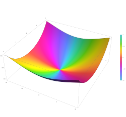
Anger function

In mathematics, the Anger function, introduced by C. T. Anger (1855), is a function defined as

${\displaystyle \mathbf {J} _{\nu }(z)={\frac {1}{\pi }}\int _{0}^{\pi }\cos(\nu \theta -z\sin \theta )\,d\theta }$

with complex parameter ${\displaystyle \nu }$ and complex variable ⁠${\displaystyle {\textit {z}}}$⁠.¹ It is closely related to the Bessel functions.

The Weber function (also known as Lommel–Weber function), introduced by H. F. Weber (1879), is a closely related function defined by

${\displaystyle \mathbf {E} _{\nu }(z)={\frac {1}{\pi }}\int _{0}^{\pi }\sin(\nu \theta -z\sin \theta )\,d\theta }$

and is closely related to Bessel functions of the second kind.

The Anger and Weber functions are related by

${\displaystyle {\begin{aligned}\sin(\pi \nu )\mathbf {J} _{\nu }(z)&=\cos(\pi \nu )\mathbf {E} _{\nu }(z)-\mathbf {E} _{-\nu }(z),\\-\sin(\pi \nu )\mathbf {E} _{\nu }(z)&=\cos(\pi \nu )\mathbf {J} _{\nu }(z)-\mathbf {J} _{-\nu }(z),\end{aligned}}}$

so in particular if ν is not an integer they can be expressed as linear combinations of each other. If ν is an integer then Anger functions J_ν are the same as Bessel functions J_ν, and Weber functions can be expressed as finite linear combinations of Struve functions.

The Anger function has the power series expansion²

${\displaystyle \mathbf {J} _{\nu }(z)=\cos {\frac {\pi \nu }{2}}\sum _{k=0}^{\infty }{\frac {(-1)^{k}z^{2k}}{4^{k}\Gamma \left(k+{\frac {\nu }{2}}+1\right)\Gamma \left(k-{\frac {\nu }{2}}+1\right)}}+\sin {\frac {\pi \nu }{2}}\sum _{k=0}^{\infty }{\frac {(-1)^{k}z^{2k+1}}{2^{2k+1}\Gamma \left(k+{\frac {\nu }{2}}+{\frac {3}{2}}\right)\Gamma \left(k-{\frac {\nu }{2}}+{\frac {3}{2}}\right)}}.}$

While the Weber function has the power series expansion²

${\displaystyle \mathbf {E} _{\nu }(z)=\sin {\frac {\pi \nu }{2}}\sum _{k=0}^{\infty }{\frac {(-1)^{k}z^{2k}}{4^{k}\Gamma \left(k+{\frac {\nu }{2}}+1\right)\Gamma \left(k-{\frac {\nu }{2}}+1\right)}}-\cos {\frac {\pi \nu }{2}}\sum _{k=0}^{\infty }{\frac {(-1)^{k}z^{2k+1}}{2^{2k+1}\Gamma \left(k+{\frac {\nu }{2}}+{\frac {3}{2}}\right)\Gamma \left(k-{\frac {\nu }{2}}+{\frac {3}{2}}\right)}}.}$

The Anger and Weber functions are solutions of inhomogeneous forms of Bessel's equation

${\displaystyle z^{2}y^{\prime \prime }+zy^{\prime }+(z^{2}-\nu ^{2})y=0.}$

More precisely, the Anger functions satisfy the equation²

${\displaystyle z^{2}y^{\prime \prime }+zy^{\prime }+(z^{2}-\nu ^{2})y={\frac {(z-\nu )\sin(\pi \nu )}{\pi }},}$

and the Weber functions satisfy the equation²

${\displaystyle z^{2}y^{\prime \prime }+zy^{\prime }+(z^{2}-\nu ^{2})y=-{\frac {z+\nu +(z-\nu )\cos(\pi \nu )}{\pi }}.}$

The Anger function satisfies this inhomogeneous form of recurrence relation²

${\displaystyle z\mathbf {J} _{\nu -1}(z)+z\mathbf {J} _{\nu +1}(z)=2\nu \mathbf {J} _{\nu }(z)-{\frac {2\sin \pi \nu }{\pi }}.}$

While the Weber function satisfies this inhomogeneous form of recurrence relation²

${\displaystyle z\mathbf {E} _{\nu -1}(z)+z\mathbf {E} _{\nu +1}(z)=2\nu \mathbf {E} _{\nu }(z)-{\frac {2(1-\cos \pi \nu )}{\pi }}.}$

The Anger and Weber functions satisfy these homogeneous forms of delay differential equations²

${\displaystyle \mathbf {J} _{\nu -1}(z)-\mathbf {J} _{\nu +1}(z)=2{\dfrac {\partial }{\partial z}}\mathbf {J} _{\nu }(z),}$

${\displaystyle \mathbf {E} _{\nu -1}(z)-\mathbf {E} _{\nu +1}(z)=2{\dfrac {\partial }{\partial z}}\mathbf {E} _{\nu }(z).}$

The Anger and Weber functions also satisfy these inhomogeneous forms of delay differential equations²

${\displaystyle z{\dfrac {\partial }{\partial z}}\mathbf {J} _{\nu }(z)\pm \nu \mathbf {J} _{\nu }(z)=\pm z\mathbf {J} _{\nu \mp 1}(z)\pm {\frac {\sin \pi \nu }{\pi }},}$

${\displaystyle z{\dfrac {\partial }{\partial z}}\mathbf {E} _{\nu }(z)\pm \nu \mathbf {E} _{\nu }(z)=\pm z\mathbf {E} _{\nu \mp 1}(z)\pm {\frac {1-\cos \pi \nu }{\pi }}.}$

References

Prudnikov, A.P. (2001) [1994], "Anger function" , Encyclopedia of Mathematics EMS Press
Paris, R. B. (2010), "Anger–Weber Functions" , in Olver, Frank W. J. ; Lozier, Daniel M.; Boisvert, Ronald F.; Clark, Charles W. (eds.), NIST Handbook of Mathematical Functions ISBN 978-0-521-19225-5 MR 2723248
Abramowitz, Milton ; Stegun, Irene Ann , eds. (1983) [June 1964]. "Chapter 12" . Handbook of Mathematical Functions with Formulas, Graphs, and Mathematical Tables ISBN 978-0-486-61272-0 LCCN 64-60036 . MR 0167642 . LCCN 65-12253 .C.T. Anger, Neueste Schr. d. Naturf. d. Ges. i. Danzig, 5 (1855) pp. 1–29
Prudnikov, A.P. (2001) [1994], "Weber function" , Encyclopedia of Mathematics EMS Press Watson, G.N. (1952), A treatise on the theory of Bessel functions , Cambridge Univ. Press, pp. 1– 2H.F. Weber, Zurich Vierteljahresschrift, 24 (1879) pp. 33–76