Article · Wikipedia archive · Last revised Jun 16, 2026

Swap test

The swap test is a procedure in quantum computation that is used to check how much two quantum states differ, appearing first in the work of Barenco et al. and later rediscovered by Harry Buhrman, Richard Cleve, John Watrous, and Ronald de Wolf. It appears commonly in quantum machine learning, and is a circuit used for proofs-of-concept in implementations of quantum computers.

Last revised
Jun 16, 2026
Read time
≈ 5 min
Length
1,174 w
Citations
7
Source
Circuit implementing the swap test between two states | ϕ {\displaystyle |\phi \rangle } and | ψ {\displaystyle |\psi \rangle } source ↗

The swap test is a procedure in quantum computation that is used to check how much two quantum states differ, appearing first in the work of Barenco et al.1 and later rediscovered by Harry Buhrman, Richard Cleve, John Watrous, and Ronald de Wolf.2 It appears commonly in quantum machine learning, and is a circuit used for proofs-of-concept in implementations of quantum computers.34

Formally, the swap test takes two input states | ϕ {\displaystyle |\phi \rangle } and | ψ {\displaystyle |\psi \rangle } and outputs a Bernoulli random variable that is 1 with probability 1 2 1 2 | ψ | ϕ | 2 {\displaystyle \textstyle {\frac {1}{2}}-{\frac {1}{2}}{|\langle \psi |\phi \rangle |}^{2}} (where the expressions here use bra–ket notation). This allows one to, for example, estimate the squared inner product between the two states, | ψ | ϕ | 2 {\displaystyle {|\langle \psi |\phi \rangle |}^{2}} , to ε {\displaystyle \varepsilon } additive error by taking the average over O ( 1 ε 2 ) {\displaystyle O(\textstyle {\frac {1}{\varepsilon ^{2}}})} runs of the swap test.5 This requires O ( 1 ε 2 ) {\displaystyle O(\textstyle {\frac {1}{\varepsilon ^{2}}})} copies of the input states. The squared inner product roughly measures "overlap" between the two states, and can be used in linear-algebraic applications, including clustering quantum states.6

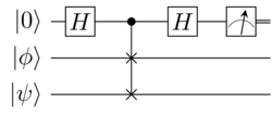
Explanation of the circuit

Consider two states: | ϕ {\displaystyle |\phi \rangle } and | ψ {\displaystyle |\psi \rangle } . The state of the system at the beginning of the protocol is | 0 , ϕ , ψ {\displaystyle |0,\phi ,\psi \rangle } . After the Hadamard gate, the state of the system is 1 2 ( | 0 , ϕ , ψ + | 1 , ϕ , ψ ) {\displaystyle {\frac {1}{\sqrt {2}}}(|0,\phi ,\psi \rangle +|1,\phi ,\psi \rangle )} . The controlled SWAP gate transforms the state into 1 2 ( | 0 , ϕ , ψ + | 1 , ψ , ϕ ) {\displaystyle {\frac {1}{\sqrt {2}}}(|0,\phi ,\psi \rangle +|1,\psi ,\phi \rangle )} . The second Hadamard gate results in 1 2 ( | 0 , ϕ , ψ + | 1 , ϕ , ψ + | 0 , ψ , ϕ | 1 , ψ , ϕ ) = 1 2 | 0 ( | ϕ , ψ + | ψ , ϕ ) + 1 2 | 1 ( | ϕ , ψ | ψ , ϕ ) {\displaystyle {\frac {1}{2}}(|0,\phi ,\psi \rangle +|1,\phi ,\psi \rangle +|0,\psi ,\phi \rangle -|1,\psi ,\phi \rangle )={\frac {1}{2}}|0\rangle (|\phi ,\psi \rangle +|\psi ,\phi \rangle )+{\frac {1}{2}}|1\rangle (|\phi ,\psi \rangle -|\psi ,\phi \rangle )}

The measurement gate on the first qubit ensures that it's 0 with a probability of

P ( First qubit = 0 ) = 1 2 ( ϕ | ψ | + ψ | ϕ | ) 1 2 ( | ϕ | ψ + | ψ | ϕ ) = 1 2 + 1 2 | ψ | ϕ | 2 {\displaystyle P({\text{First qubit}}=0)={\frac {1}{2}}{\Big (}\langle \phi |\langle \psi |+\langle \psi |\langle \phi |{\Big )}{\frac {1}{2}}{\Big (}|\phi \rangle |\psi \rangle +|\psi \rangle |\phi \rangle {\Big )}={\frac {1}{2}}+{\frac {1}{2}}{|\langle \psi |\phi \rangle |}^{2}}

when measured. If ψ {\displaystyle \psi } and ϕ {\displaystyle \phi } are orthogonal ( | ψ | ϕ | 2 = 0 ) {\displaystyle ({|\langle \psi |\phi \rangle |}^{2}=0)} , then the probability that 0 is measured is 1 2 {\displaystyle {\frac {1}{2}}} . If the states are equal ( | ψ | ϕ | 2 = 1 ) {\displaystyle ({|\langle \psi |\phi \rangle |}^{2}=1)} , then the probability that 0 is measured is 1.2

In general, for P {\displaystyle P} trials of the swap test using P {\displaystyle P} copies of | ϕ {\displaystyle |\phi \rangle } and P {\displaystyle P} copies of | ψ {\displaystyle |\psi \rangle } , the fraction of measurements that are zero is 1 1 P i = 1 P M i {\displaystyle 1-\textstyle {\frac {1}{P}}\textstyle \sum _{i=1}^{P}M_{i}} , so by taking P {\displaystyle P\rightarrow \infty } , one can get arbitrary precision of this value.

Below is the pseudocode for estimating the value of | ψ | ϕ | 2 {\displaystyle |\langle \psi |\phi \rangle |^{2}} using P copies of | ψ {\displaystyle |\psi \rangle } and | ϕ {\displaystyle |\phi \rangle } :

Inputs P copies each of the n qubits quantum states 


          |
        
        ψ


    {\displaystyle |\psi \rangle }
  
 and 


          |
        
        ϕ


    {\displaystyle |\phi \rangle }
  

Output An estimate of 


          |
        
        
        ψ
        
          |
        
        ϕ


            |
          
          
            2


    {\displaystyle |\langle \psi |\phi \rangle |^{2}}


for j ranging from 1 to P:
    initialize an ancilla qubit A in state 


          |
        
        0


    {\displaystyle |0\rangle }
  

    apply a Hadamard gate to the ancilla qubit A
    for i ranging from 1 to n: 
        apply CSWAP to 


          ψ
          
            i


    {\displaystyle \psi _{i}}
  
 and 


          ϕ
          
            i


    {\displaystyle \phi _{i}}
  
 (the ith qubit of the jth copy of 


          |
        
        ψ


    {\displaystyle |\psi \rangle }
  
 and 


          |
        
        ϕ


    {\displaystyle |\phi \rangle }
  
), with A as the control qubit
    apply a Hadamard gate to the ancilla qubit A
    measure A in the 


        Z
      
    
    {\displaystyle Z}
  
 basis and record the measurement Mj as either a 0 or 1
compute 


        s
        =
        1


              2
              P


                i
                =
                1
              
              
                P


              M
              
                i


    {\displaystyle s=1-\textstyle {\frac {2}{P}}\textstyle \sum _{i=1}^{P}M_{i}}
  
.
return 


        s
      
    
    {\displaystyle s}
  
 as our estimate of 


          |
        
        
        ψ
        
          |
        
        ϕ


            |
          
          
            2


    {\displaystyle |\langle \psi |\phi \rangle |^{2}}
  

References

References

  1. Adriano Barenco, André Berthiaume, David Deutsch, Artur Ekert, Richard Jozsa, Chiara Macchiavello (1997). "Stabilization of Quantum Computations by Symmetrization". SIAM Journal on Computing. 26 (5): 1541–1557. arXiv:quant-ph/9604028. doi:10.1137/S0097539796302452.{{cite journal}}: CS1 maint: multiple names: authors list (link)
  2. Harry Buhrman, Richard Cleve, John Watrous, Ronald de Wolf (2001). "Quantum Fingerprinting". Physical Review Letters. 87 (16) 167902. arXiv:quant-ph/0102001. Bibcode:2001PhRvL..87p7902B. doi:10.1103/PhysRevLett.87.167902. PMID 11690244. S2CID 1096490.{{cite journal}}: CS1 maint: multiple names: authors list (link)
  3. Schuld, Maria; Sinayskiy, Ilya; Petruccione, Francesco (2015-04-03). "An introduction to quantum machine learning". Contemporary Physics. 56 (2): 172–185. arXiv:1409.3097. Bibcode:2015ConPh..56..172S. doi:10.1080/00107514.2014.964942. ISSN 0010-7514. S2CID 119263556.
  4. Kang Min-Sung, Heo Jino, Choi Seong-Gon, Moon Sung, Han Sang-Wook (2019). "Implementation of SWAP test for two unknown states in photons via cross-Kerr nonlinearities under decoherence effect". Scientific Reports. 9 (1): 6167. Bibcode:2019NatSR...9.6167K. doi:10.1038/s41598-019-42662-4. PMC 6468003. PMID 30992536.{{cite journal}}: CS1 maint: multiple names: authors list (link)
  5. de Wolf, Ronald (2021-01-20). "Quantum Computing: Lecture Notes". pp. 117–119, 122. arXiv:1907.09415 [quant-ph].
  6. Wiebe, Nathan; Kapoor, Anish; Svore, Krysta M. (1 March 2015). "Quantum Algorithms for Nearest-Neighbor Methods for Supervised and Unsupervised Learning". Quantum Information and Computation. 15 (3–4). Rinton Press, Incorporated: 316–356. arXiv:1401.2142. doi:10.26421/QIC15.3-4-7. S2CID 37339559.