Article · Wikipedia archive · Last revised Jul 15, 2026

Padua points

In polynomial interpolation of two variables, the Padua points are the first known example of a unisolvent point set with minimal growth of their Lebesgue constant, proven to be . Their name is due to the University of Padua, where they were originally discovered.

Last revised
Jul 15, 2026
Read time
≈ 7 min
Length
1,638 w
Citations
5
Source

In polynomial interpolation of two variables, the Padua points are the first known example (and up to now the only one) of a unisolvent point set (that is, the interpolating polynomial is unique) with minimal growth of their Lebesgue constant, proven to be O ( log 2 n ) {\displaystyle O(\log ^{2}n)} .1 Their name is due to the University of Padua, where they were originally discovered.2

The points are defined in the domain [ 1 , 1 ] × [ 1 , 1 ] R 2 {\displaystyle [-1,1]\times [-1,1]\subset \mathbb {R} ^{2}} . It is possible to use the points with four orientations, obtained with subsequent 90-degree rotations: this way we get four different families of Padua points.

The four families

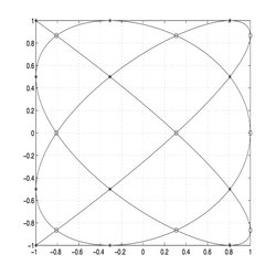
Padua points of the first family and of degree 5, plotted with their generating curve. source ↗
Padua points of the first family and of degree 6, plotted with their generating curve. source ↗

We can see the Padua point as a "sampling" of a parametric curve, called generating curve, which is slightly different for each of the four families, so that the points for interpolation degree n {\displaystyle n} and family s {\displaystyle s} can be defined as

Pad n s = { ξ = ( ξ 1 , ξ 2 ) } = { γ s ( k π n ( n + 1 ) ) , k = 0 , , n ( n + 1 ) } . {\displaystyle {\text{Pad}}_{n}^{s}=\lbrace \mathbf {\xi } =(\xi _{1},\xi _{2})\rbrace =\left\lbrace \gamma _{s}\left({\frac {k\pi }{n(n+1)}}\right),k=0,\ldots ,n(n+1)\right\rbrace .}

Actually, the Padua points lie exactly on the self-intersections of the curve, and on the intersections of the curve with the boundaries of the square [ 1 , 1 ] 2 {\displaystyle [-1,1]^{2}} . The cardinality of the set Pad n s {\displaystyle \operatorname {Pad} _{n}^{s}} is | Pad n s | = ( n + 1 ) ( n + 2 ) 2 {\textstyle |\operatorname {Pad} _{n}^{s}|={\frac {(n+1)(n+2)}{2}}} . Moreover, for each family of Padua points, two points lie on consecutive vertices of the square [ 1 , 1 ] 2 {\displaystyle [-1,1]^{2}} , 2 n 1 {\displaystyle 2n-1} points lie on the edges of the square, and the remaining points lie on the self-intersections of the generating curve inside the square.34

The four generating curves are closed parametric curves in the interval [ 0 , 2 π ] {\displaystyle [0,2\pi ]} , and are a special case of Lissajous curves.

The first family

The generating curve of Padua points of the first family is

γ 1 ( t ) = [ cos ( ( n + 1 ) t ) , cos ( n t ) ] , t [ 0 , π ] . {\displaystyle \gamma _{1}(t)=[-\cos((n+1)t),-\cos(nt)],\quad t\in [0,\pi ].}

If we sample it as written above, we have:

Pad n 1 = { ξ = ( μ j , η k ) , 0 j n ; 1 k n 2 + 1 + δ j } , {\displaystyle \operatorname {Pad} _{n}^{1}=\lbrace \mathbf {\xi } =(\mu _{j},\eta _{k}),0\leq j\leq n;1\leq k\leq \lfloor {\frac {n}{2}}\rfloor +1+\delta _{j}\rbrace ,}

where δ j = 0 {\displaystyle \delta _{j}=0} when n {\displaystyle n} is even or odd but j {\displaystyle j} is even, δ j = 1 {\displaystyle \delta _{j}=1} if n {\displaystyle n} and k {\displaystyle k} are both odd

with

μ j = cos ( j π n ) , η k = { cos ( ( 2 k 2 ) π n + 1 ) j  odd cos ( ( 2 k 1 ) π n + 1 ) j  even. {\displaystyle \mu _{j}=\cos \left({\frac {j\pi }{n}}\right),\eta _{k}={\begin{cases}\cos \left({\frac {(2k-2)\pi }{n+1}}\right)&j{\mbox{ odd}}\\\cos \left({\frac {(2k-1)\pi }{n+1}}\right)&j{\mbox{ even.}}\end{cases}}}

From this follows that the Padua points of first family will have two vertices on the bottom if n {\displaystyle n} is even, or on the left if n {\displaystyle n} is odd.

The second family

The generating curve of Padua points of the second family is

γ 2 ( t ) = [ cos ( n t ) , cos ( ( n + 1 ) t ) ] , t [ 0 , π ] , {\displaystyle \gamma _{2}(t)=[-\cos(nt),-\cos((n+1)t)],\quad t\in [0,\pi ],}

which leads to have vertices on the left if n {\displaystyle n} is even and on the bottom if n {\displaystyle n} is odd.

The third family

The generating curve of Padua points of the third family is

γ 3 ( t ) = [ cos ( ( n + 1 ) t ) , cos ( n t ) ] , t [ 0 , π ] , {\displaystyle \gamma _{3}(t)=[\cos((n+1)t),\cos(nt)],\quad t\in [0,\pi ],}

which leads to have vertices on the top if n {\displaystyle n} is even and on the right if n {\displaystyle n} is odd.

The fourth family

The generating curve of Padua points of the fourth family is

γ 4 ( t ) = [ cos ( n t ) , cos ( ( n + 1 ) t ) ] , t [ 0 , π ] , {\displaystyle \gamma _{4}(t)=[\cos(nt),\cos((n+1)t)],\quad t\in [0,\pi ],}

which leads to have vertices on the right if n {\displaystyle n} is even and on the top if n {\displaystyle n} is odd.

The interpolation formula

The explicit representation of their fundamental Lagrange polynomial is based on the reproducing kernel K n ( x , y ) {\displaystyle K_{n}(\mathbf {x} ,\mathbf {y} )} , x = ( x 1 , x 2 ) {\displaystyle \mathbf {x} =(x_{1},x_{2})} and y = ( y 1 , y 2 ) {\displaystyle \mathbf {y} =(y_{1},y_{2})} , of the space Π n 2 ( [ 1 , 1 ] 2 ) {\displaystyle \Pi _{n}^{2}([-1,1]^{2})} equipped with the inner product

f , g = 1 π 2 [ 1 , 1 ] 2 f ( x 1 , x 2 ) g ( x 1 , x 2 ) d x 1 1 x 1 2 d x 2 1 x 2 2 {\displaystyle \langle f,g\rangle ={\frac {1}{\pi ^{2}}}\int _{[-1,1]^{2}}f(x_{1},x_{2})g(x_{1},x_{2}){\frac {dx_{1}}{\sqrt {1-x_{1}^{2}}}}{\frac {dx_{2}}{\sqrt {1-x_{2}^{2}}}}}

defined by

K n ( x , y ) = k = 0 n j = 0 k T ^ j ( x 1 ) T ^ k j ( x 2 ) T ^ j ( y 1 ) T ^ k j ( y 2 ) {\displaystyle K_{n}(\mathbf {x} ,\mathbf {y} )=\sum _{k=0}^{n}\sum _{j=0}^{k}{\hat {T}}_{j}(x_{1}){\hat {T}}_{k-j}(x_{2}){\hat {T}}_{j}(y_{1}){\hat {T}}_{k-j}(y_{2})}

with T ^ j {\displaystyle {\hat {T}}_{j}} representing the normalized Chebyshev polynomial of degree j {\displaystyle j} (that is, T ^ 0 = T 0 {\displaystyle {\hat {T}}_{0}=T_{0}} and T ^ p = 2 T p {\displaystyle {\hat {T}}_{p}={\sqrt {2}}T_{p}} , where T p ( ) = cos ( p arccos ( ) ) {\displaystyle T_{p}(\cdot )=\cos(p\arccos(\cdot ))} is the classical Chebyshev polynomial of first kind of degree p {\displaystyle p} ).3 For the four families of Padua points, which we may denote by Pad n s = { ξ = ( ξ 1 , ξ 2 ) } {\displaystyle \operatorname {Pad} _{n}^{s}=\lbrace \mathbf {\xi } =(\xi _{1},\xi _{2})\rbrace } , s = { 1 , 2 , 3 , 4 } {\displaystyle s=\lbrace 1,2,3,4\rbrace } , the interpolation formula of order n {\displaystyle n} of the function f : [ 1 , 1 ] 2 R 2 {\displaystyle f\colon [-1,1]^{2}\to \mathbb {R} ^{2}} on the generic target point x [ 1 , 1 ] 2 {\displaystyle \mathbf {x} \in [-1,1]^{2}} is then

L n s f ( x ) = ξ Pad n s f ( ξ ) L ξ s ( x ) {\displaystyle {\mathcal {L}}_{n}^{s}f(\mathbf {x} )=\sum _{\mathbf {\xi } \in \operatorname {Pad} _{n}^{s}}f(\mathbf {\xi } )L_{\mathbf {\xi } }^{s}(\mathbf {x} )}

where L ξ s ( x ) {\displaystyle L_{\mathbf {\xi } }^{s}(\mathbf {x} )} is the fundamental Lagrange polynomial

L ξ s ( x ) = w ξ ( K n ( ξ , x ) T n ( ξ i ) T n ( x i ) ) , s = 1 , 2 , 3 , 4 , i = 2 ( s mod 2 ) . {\displaystyle L_{\mathbf {\xi } }^{s}(\mathbf {x} )=w_{\mathbf {\xi } }(K_{n}(\mathbf {\xi } ,\mathbf {x} )-T_{n}(\xi _{i})T_{n}(x_{i})),\quad s=1,2,3,4,\quad i=2-(s\mod 2).}

The weights w ξ {\displaystyle w_{\mathbf {\xi } }} are defined as

w ξ = 1 n ( n + 1 ) { 1 2  if  ξ  is a vertex point 1  if  ξ  is an edge point 2  if  ξ  is an interior point. {\displaystyle w_{\mathbf {\xi } }={\frac {1}{n(n+1)}}\cdot {\begin{cases}{\frac {1}{2}}{\text{ if }}\mathbf {\xi } {\text{ is a vertex point}}\\1{\text{ if }}\mathbf {\xi } {\text{ is an edge point}}\\2{\text{ if }}\mathbf {\xi } {\text{ is an interior point.}}\end{cases}}}
References

References

  1. Caliari, Marco; Bos, Len; de Marchi, Stefano; Vianello, Marco; Xu, Yuan (2006), "Bivariate Lagrange interpolation at the Padua points: the generating curve approach", J. Approx. Theory, 143 (1): 15–25, arXiv:math/0604604, doi:10.1016/j.jat.2006.03.008
  2. de Marchi, Stefano; Caliari, Marco; Vianello, Marco (2005), "Bivariate polynomial interpolation at new nodal sets", Appl. Math. Comput., 165 (2): 261–274, doi:10.1016/j.amc.2004.07.001
  3. Caliari, Marco; de Marchi, Stefano; Vianello, Marco (2008), "Algorithm 886: Padua2D—Lagrange Interpolation at Padua Points on Bivariate Domains", ACM Transactions on Mathematical Software, 35 (3): 1–11, doi:10.1145/1391989.1391994
  4. Bos, Len; de Marchi, Stefano; Vianello, Marco; Xu, Yuan (2007), "Bivariate Lagrange interpolation at the Padua points: the ideal theory approach", Numerische Mathematik, 108 (1): 43–57, arXiv:math/0604604, doi:10.1007/s00211-007-0112-z
External links