Article · Wikipedia archive · Last revised Jul 19, 2026

Lax–Wendroff method

The Lax–Wendroff method, named after Peter Lax and Burton Wendroff, is a numerical method for the solution of hyperbolic partial differential equations, based on finite differences. It is second-order accurate in both space and time. This method is an example of explicit time integration where the function that defines the governing equation is evaluated at the current time.

Last revised
Jul 19, 2026
Read time
≈ 4 min
Length
935 w
Citations
2
Source
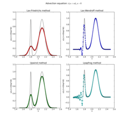
Graphs that show different Lax–Wendroff methods source ↗

The Lax–Wendroff method, named after Peter Lax and Burton Wendroff,1 is a numerical method for the solution of hyperbolic partial differential equations, based on finite differences. It is second-order accurate in both space and time. This method is an example of explicit time integration where the function that defines the governing equation is evaluated at the current time.

Definition

Suppose one has an equation of the following form: u ( x , t ) t + f ( u ( x , t ) ) x = 0 {\displaystyle {\frac {\partial u(x,t)}{\partial t}}+{\frac {\partial f(u(x,t))}{\partial x}}=0} where x and t are independent variables, and the initial state, u(x, 0) is given.

Linear case

In the linear case, where f(u) = Au, and A is a constant,2 u i n + 1 = u i n Δ t 2 Δ x A [ u i + 1 n u i 1 n ] + Δ t 2 2 Δ x 2 A 2 [ u i + 1 n 2 u i n + u i 1 n ] . {\displaystyle u_{i}^{n+1}=u_{i}^{n}-{\frac {\Delta t}{2\Delta x}}A\left[u_{i+1}^{n}-u_{i-1}^{n}\right]+{\frac {\Delta t^{2}}{2\Delta x^{2}}}A^{2}\left[u_{i+1}^{n}-2u_{i}^{n}+u_{i-1}^{n}\right].} Here n {\displaystyle n} refers to the t {\displaystyle t} dimension and i {\displaystyle i} refers to the x {\displaystyle x} dimension. This linear scheme can be extended to the general non-linear case in different ways. One of them is letting A ( u ) = f ( u ) = f u {\displaystyle A(u)=f'(u)={\frac {\partial f}{\partial u}}}

Non-linear case

The conservative form of Lax-Wendroff for a general non-linear equation is then: u i n + 1 = u i n Δ t 2 Δ x [ f ( u i + 1 n ) f ( u i 1 n ) ] + Δ t 2 2 Δ x 2 [ A i + 1 / 2 ( f ( u i + 1 n ) f ( u i n ) ) A i 1 / 2 ( f ( u i n ) f ( u i 1 n ) ) ] . {\displaystyle u_{i}^{n+1}=u_{i}^{n}-{\frac {\Delta t}{2\Delta x}}\left[f(u_{i+1}^{n})-f(u_{i-1}^{n})\right]+{\frac {\Delta t^{2}}{2\Delta x^{2}}}\left[A_{i+1/2}\left(f(u_{i+1}^{n})-f(u_{i}^{n})\right)-A_{i-1/2}\left(f(u_{i}^{n})-f(u_{i-1}^{n})\right)\right].} where A i ± 1 / 2 {\displaystyle A_{i\pm 1/2}} is the Jacobian matrix evaluated at 1 2 ( u i n + u i ± 1 n ) {\textstyle {\frac {1}{2}}(u_{i}^{n}+u_{i\pm 1}^{n})} .

Jacobian free methods

To avoid the Jacobian evaluation, use a two-step procedure.

Richtmyer method

What follows is the Richtmyer two-step Lax–Wendroff method. The first step in the Richtmyer two-step Lax–Wendroff method calculates values for f(u(x, t)) at half time steps, tn + 1/2 and half grid points, xi + 1/2. In the second step values at tn + 1 are calculated using the data for tn and tn + 1/2.

First (Lax) steps: u i + 1 / 2 n + 1 / 2 = 1 2 ( u i + 1 n + u i n ) Δ t 2 Δ x ( f ( u i + 1 n ) f ( u i n ) ) , {\displaystyle u_{i+1/2}^{n+1/2}={\frac {1}{2}}(u_{i+1}^{n}+u_{i}^{n})-{\frac {\Delta t}{2\,\Delta x}}(f(u_{i+1}^{n})-f(u_{i}^{n})),} u i 1 / 2 n + 1 / 2 = 1 2 ( u i n + u i 1 n ) Δ t 2 Δ x ( f ( u i n ) f ( u i 1 n ) ) . {\displaystyle u_{i-1/2}^{n+1/2}={\frac {1}{2}}(u_{i}^{n}+u_{i-1}^{n})-{\frac {\Delta t}{2\,\Delta x}}(f(u_{i}^{n})-f(u_{i-1}^{n})).}

Second step: u i n + 1 = u i n Δ t Δ x [ f ( u i + 1 / 2 n + 1 / 2 ) f ( u i 1 / 2 n + 1 / 2 ) ] . {\displaystyle u_{i}^{n+1}=u_{i}^{n}-{\frac {\Delta t}{\Delta x}}\left[f(u_{i+1/2}^{n+1/2})-f(u_{i-1/2}^{n+1/2})\right].}

MacCormack method

Another method of this same type was proposed by MacCormack. MacCormack's method uses first forward differencing and then backward differencing:

First step: u i = u i n Δ t Δ x ( f ( u i + 1 n ) f ( u i n ) ) . {\displaystyle u_{i}^{*}=u_{i}^{n}-{\frac {\Delta t}{\Delta x}}(f(u_{i+1}^{n})-f(u_{i}^{n})).} Second step: u i n + 1 = 1 2 ( u i n + u i ) Δ t 2 Δ x [ f ( u i ) f ( u i 1 ) ] . {\displaystyle u_{i}^{n+1}={\frac {1}{2}}(u_{i}^{n}+u_{i}^{*})-{\frac {\Delta t}{2\Delta x}}\left[f(u_{i}^{*})-f(u_{i-1}^{*})\right].}

Alternatively, First step: u i = u i n Δ t Δ x ( f ( u i n ) f ( u i 1 n ) ) . {\displaystyle u_{i}^{*}=u_{i}^{n}-{\frac {\Delta t}{\Delta x}}(f(u_{i}^{n})-f(u_{i-1}^{n})).} Second step: u i n + 1 = 1 2 ( u i n + u i ) Δ t 2 Δ x [ f ( u i + 1 ) f ( u i ) ] . {\displaystyle u_{i}^{n+1}={\frac {1}{2}}(u_{i}^{n}+u_{i}^{*})-{\frac {\Delta t}{2\Delta x}}\left[f(u_{i+1}^{*})-f(u_{i}^{*})\right].}

References

References

  1. P.D Lax; B. Wendroff (1960). "Systems of conservation laws" (PDF). Commun. Pure Appl. Math. 13 (2): 217–237. doi:10.1002/cpa.3160130205. Archived from the original on September 25, 2017.
  2. LeVeque, Randall J. (1992). Numerical Methods for Conservation Laws (PDF). Boston: Birkhäuser. p. 125. ISBN 0-8176-2723-5.