| Inverse Gaussian | |||
|---|---|---|---|
|
Probability density function 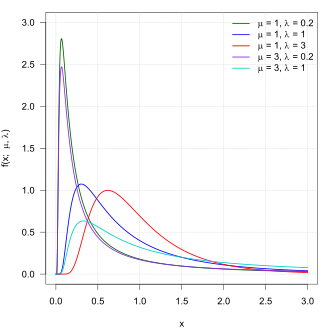 | |||
|
Cumulative distribution function 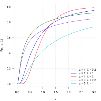 | |||
| Notation | |||
| Parameters |
| ||
| Support | |||
| CDF |
where is the standard normal (standard Gaussian) distribution c.d.f. | ||
| Mean |
| ||
| Mode | |||
| Variance |
| ||
| Skewness | |||
| Excess kurtosis | |||
| MGF | |||
| CF | |||
In probability theory, the inverse Gaussian distribution (also known as the Wald distribution) is a two-parameter family of continuous probability distributions with support on .
Its probability density function is given by
for , where is the mean and is a shape parameter.1 Either or (or more generally any combination of the form for any real ) can serve as a scale parameter, so a proper (i.e., unscaled) shape parameter would be any non-zero power of : Tweedie proposed to use the and parametrizations in addition to the standard parametrization (“Each of these forms is convenient or suggestive for some purpose.”2), and later on uses exclusively the parametrization.3
The inverse Gaussian distribution has several properties analogous to a Gaussian distribution. The name can be misleading: it is an inverse only in that, while the Gaussian describes a Brownian motion's level at a fixed time, the inverse Gaussian describes the distribution of the time a Brownian motion with positive drift takes to reach a fixed positive level. The relationship between the Gaussian and inverse Gaussian distributions is thus the same as the relationship between the binomial (number of successes for a fixed number of Bernoulli trials) and negative binomial (number of Bernoulli trials for a fixed number of successes) distributions.4
The y-axis reflections of the cumulant generating functions of the Gaussian and inverse Gaussian distributions are inverse of each other (i.e., the graphs of the two cumulant generating functions are reflections of each other across the line ), a property that is also shared between the binomial and negative binomial distributions (after dividing their cumulant generating functions by their respective fixed parameter).4
To indicate that a random variable is inverse Gaussian-distributed with mean and shape parameter we write .
Properties
Single parameter form
The probability density function (pdf) of the inverse Gaussian distribution has a single parameter form given by
In this form, the mean and variance of the distribution are equal, .
Also, the cumulative distribution function (cdf) of the single parameter inverse Gaussian distribution is related to the standard normal distribution by
where , , and the is the cdf of standard normal distribution. The variables and are related to each other by the identity .
In the single parameter form, the MGF simplifies to
An inverse Gaussian distribution in double parameter form can be transformed into a single parameter form by appropriate scaling , where .
The above paragraph can be re-written as: if , then 5. This approach is better in the sense that it clearly shows dimensionless nature of the single parameter form (note that ). This property follows from a more general fact: if and , then 2.
The standard form of inverse Gaussian distribution is
Summation
If has an distribution for and all are independent, then
The special case shows that the inverse Gaussian distribution is infinitely divisible.
Note that
is constant for all . This is a necessary condition for the summation. Otherwise would not be Inverse Gaussian distributed.
Scaling
For any it holds that
Exponential family
The inverse Gaussian distribution is a two-parameter exponential family with natural parameters and , and natural statistics and .
For fixed, it is also a single-parameter natural exponential family distribution6 where the base distribution has density
Indeed, with ,
is a density over the reals. Evaluating the integral, we get
Substituting makes the above expression equal to .
Relationship with Brownian motion
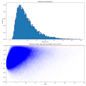
Let the stochastic process be given by
where is a standard Brownian motion. That is, is a Brownian motion with drift .
Then the first passage time for a fixed level by is distributed according to an inverse-Gaussian:
i.e
(cf. Schrödinger7 equation 19, Smoluchowski8, equation 8, and Folks5, equation 1).
Derivation of the first passage time distribution
|
|---|
|
Suppose that we have a Brownian motion with drift defined by: And suppose that we wish to find the probability density function for the time when the process first hits some barrier - known as the first passage time. The Fokker–Planck equation describing the evolution of the probability distribution is: where is the Dirac delta function. This is a boundary value problem (BVP) with a single absorbing boundary condition , which may be solved using the method of images. Based on the initial condition, the fundamental solution to the Fokker–Planck equation, denoted by , is: Define a point , such that . This will allow the original and mirror solutions to cancel out exactly at the barrier at each instant in time. This implies that the initial condition should be augmented to become: where is a constant. Due to the linearity of the BVP, the solution to the Fokker–Planck equation with this initial condition is: Now we must determine the value of . The fully absorbing boundary condition implies that: At , we have that . Substituting this back into the above equation, we find that: Therefore, the full solution to the BVP is: Now that we have the full probability density function, we are ready to find the first passage time distribution . The simplest route is to first compute the survival function , which is defined as: where is the cumulative distribution function of the standard normal distribution. The survival function gives us the probability that the Brownian motion process has not crossed the barrier at some time . Finally, the first passage time distribution is obtained from the identity: Assuming that , the first passage time follows an inverse Gaussian distribution: |
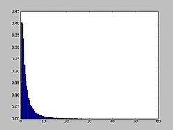
When drift is zero
A common special case of the above arises when the Brownian motion has no drift. In that case, parameter tends to infinity, and the first passage time for fixed level has probability density function
(see also Bachelier9: 74 10: 39 ). This is a Lévy distribution with parameters and .
Maximum likelihood
The model where
with all known, unknown and all independent has the following likelihood function:
Solving the likelihood equation yields the following maximum likelihood estimates
and are independent and
Sampling from an inverse-Gaussian distribution
The following algorithm may be used.11
Generate a random variate from a normal distribution with mean and standard deviation equal
Square the value
and use the relation
Generate another random variate, this time sampled from a uniform distribution between and
If then return else return
Sample code in Java:
public double inverseGaussian(double mu, double lambda) {
    Random rand = new Random();
    double v = rand.nextGaussian();  // Sample from a normal distribution with a mean of 0 and 1 standard deviation
    double y = v * v;
    double x = mu + (mu * mu * y) / (2 * lambda) - (mu / (2 * lambda)) * Math.sqrt(4 * mu * lambda * y + mu * mu * y * y);
    double test = rand.nextDouble();  // Sample from a uniform distribution between 0 and 1
    if (test <= (mu) / (mu + x))
        return x;
    else
        return (mu * mu) / x;
}
And to plot Wald distribution in Python using matplotlib and NumPy:
import matplotlib.pyplot as plt
import numpy as np

h = plt.hist(np.random.wald(3, 2, 100000), bins = 200, density = True)

plt.show()
Related distributions
The convolution of an inverse Gaussian distribution (a Wald distribution) and an exponential (an ex-Wald distribution) is used as a model for response times in psychology,13 with visual search as one example.14
History
This distribution appears to have been first derived in 1900 by Louis Bachelier910 as the time a stock reaches a certain price for the first time. In 1915 it was used independently by Erwin Schrödinger7 and Marian v. Smoluchowski8 as the time to first passage of a Brownian motion. In the field of reproduction modeling it is known as the Hadwiger function, after Hugo Hadwiger who described it in 1940.15 Abraham Wald re-derived this distribution in 194416 as the limiting form of a sample in a sequential probability ratio test. The name inverse Gaussian was proposed by Maurice Tweedie in 1945.4 Tweedie investigated this distribution in 195617 and 195723 and established some of its statistical properties. The distribution was extensively reviewed by Folks and Chhikara in 1978.5
Rated inverse Gaussian distribution
Assuming that the time intervals between occurrences of a random phenomenon follow an inverse Gaussian distribution, the probability distribution for the number of occurrences of this event within a specified time window is referred to as rated inverse Gaussian.18 While, first and second moment of this distribution are calculated, the derivation of the moment generating function remains an open problem.
Numeric computation and software
Despite the simple formula for the probability density function, numerical probability calculations for the inverse Gaussian distribution nevertheless require special care to achieve full machine accuracy in floating point arithmetic for all parameter values.19 Functions for the inverse Gaussian distribution are provided for the R programming language by several packages including rmutil,2021 SuppDists,22 STAR,23 invGauss,24 LaplacesDemon,25 and statmod.26
See also
See also
- Generalized inverse Gaussian distribution
- Tweedie distribution – The inverse Gaussian distribution is a member of the family of Tweedie exponential dispersion models
- Stopping time
References
References
- Chhikara, Raj S.; Folks, J. Leroy (1989), The Inverse Gaussian Distribution: Theory, Methodology and Applications, New York, NY, USA: Marcel Dekker, Inc, ISBN 0-8247-7997-5
- Tweedie, M. C. K. (1957). "Statistical Properties of Inverse Gaussian Distributions I". Annals of Mathematical Statistics. 28 (2): 362–377. doi:10.1214/aoms/1177706964. JSTOR 2237158.
- Tweedie, M. C. K. (1957). "Statistical Properties of Inverse Gaussian Distributions II". Annals of Mathematical Statistics. 28 (3): 696–705. doi:10.1214/aoms/1177706881. JSTOR 2237229.
- Tweedie, M. C. K. (1945). "Inverse Statistical Variates". Nature. 155 (3937): 453. Bibcode:1945Natur.155..453T. doi:10.1038/155453a0. S2CID 4113244.
- Folks, J. Leroy; Chhikara, Raj S. (1978), "The Inverse Gaussian Distribution and Its Statistical Application—A Review", Journal of the Royal Statistical Society, Series B (Methodological), 40 (3): 263–275, doi:10.1111/j.2517-6161.1978.tb01039.x, JSTOR 2984691, S2CID 125337421
- Seshadri, V. (1999), The Inverse Gaussian Distribution, Springer-Verlag, ISBN 978-0-387-98618-0
- Schrödinger, Erwin (1915), "Zur Theorie der Fall- und Steigversuche an Teilchen mit Brownscher Bewegung" [On the Theory of Fall- and Rise Experiments on Particles with Brownian Motion], Physikalische Zeitschrift (in German), 16 (16): 289–295
- Smoluchowski, Marian (1915), "Notiz über die Berechnung der Brownschen Molekularbewegung bei der Ehrenhaft-Millikanschen Versuchsanordnung" [Note on the Calculation of Brownian Molecular Motion in the Ehrenhaft-Millikan Experimental Set-up], Physikalische Zeitschrift (in German), 16 (17/18): 318–321
- Bachelier, Louis (1900), "Théorie de la spéculation" [The Theory of Speculation] (PDF), Ann. Sci. Éc. Norm. Supér. (in French), Serie 3, 17: 21–89, doi:10.24033/asens.476
- Bachelier, Louis (1900), "The Theory of Speculation", Ann. Sci. Éc. Norm. Supér., Serie 3, 17: 21–89 (Engl. translation by David R. May, 2011), doi:10.24033/asens.476
- Michael, John R.; Schucany, William R.; Haas, Roy W. (1976), "Generating Random Variates Using Transformations with Multiple Roots", The American Statistician, 30 (2): 88–90, doi:10.1080/00031305.1976.10479147, JSTOR 2683801
- Shuster, J. (1968). "On the inverse Gaussian distribution function". Journal of the American Statistical Association. 63 (4): 1514–1516. doi:10.1080/01621459.1968.10480942.
- Schwarz, Wolfgang (2001), "The ex-Wald distribution as a descriptive model of response times", Behavior Research Methods, Instruments, and Computers, 33 (4): 457–469, doi:10.3758/bf03195403, PMID 11816448
- Palmer, E. M.; Horowitz, T. S.; Torralba, A.; Wolfe, J. M. (2011). "What are the shapes of response time distributions in visual search?". Journal of Experimental Psychology: Human Perception and Performance. 37 (1): 58–71. doi:10.1037/a0020747. PMC 3062635. PMID 21090905.
- Hadwiger, H. (1940). "Eine analytische Reproduktionsfunktion für biologische Gesamtheiten". Skandinavisk Aktuarietidskrijt. 7 (3–4): 101–113. doi:10.1080/03461238.1940.10404802.
- Wald, Abraham (1944), "On Cumulative Sums of Random Variables", Annals of Mathematical Statistics, 15 (3): 283–296, doi:10.1214/aoms/1177731235, JSTOR 2236250
- Tweedie, M. C. K. (1956). "Some Statistical Properties of Inverse Gaussian Distributions". Virginia Journal of Science. New Series. 7 (3): 160–165.
- Capacity per unit cost-achieving input distribution of rated-inverse gaussian biological neuron M Nasiraee, HM Kordy, J Kazemitabar IEEE Transactions on Communications 70 (6), 3788-3803
- Giner, Göknur; Smyth, Gordon (August 2016). "statmod: Probability Calculations for the Inverse Gaussian Distribution". The R Journal. 8 (1): 339–351. arXiv:1603.06687. doi:10.32614/RJ-2016-024.
- Lindsey, James (2013-09-09). "rmutil: Utilities for Nonlinear Regression and Repeated Measurements Models".
- Swihart, Bruce; Lindsey, James (2019-03-04). "rmutil: Utilities for Nonlinear Regression and Repeated Measurements Models".
- Wheeler, Robert (2016-09-23). "SuppDists: Supplementary Distributions".
- Pouzat, Christophe (2015-02-19). "STAR: Spike Train Analysis with R".
- Gjessing, Hakon K. (2014-03-29). "Threshold regression that fits the (randomized drift) inverse Gaussian distribution to survival data".
- Hall, Byron; Hall, Martina; Statisticat, LLC; Brown, Eric; Hermanson, Richard; Charpentier, Emmanuel; Heck, Daniel; Laurent, Stephane; Gronau, Quentin F.; Singmann, Henrik (2014-03-29). "LaplacesDemon: Complete Environment for Bayesian Inference".
- Giner, Göknur; Smyth, Gordon (2017-06-18). "statmod: Statistical Modeling".
Further reading
Further reading
- Høyland, Arnljot; Rausand, Marvin (1994). System Reliability Theory. New York: Wiley. ISBN 978-0-471-59397-3.
- Seshadri, V. (1993). The Inverse Gaussian Distribution. Oxford University Press. ISBN 978-0-19-852243-0.