Extended phase graph

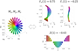
In magnetic resonance imaging and nuclear magnetic resonance the extended phase graph (EPG) is a mathematical framework used to track how magnetization evolves in a voxel through a series of radiofrequency (RF) pulses and gradients. While traditional Bloch simulations track individual spins in the spatial domain, EPG operates in the Fourier domain.² The magnetization vectors along one dimension of a voxel are stored as Fourier coefficients. Each Fourier coefficient represents the weighting of a helix that twists along one dimension of the voxel with an integer number of twists. Performing a weighted sum of all the helices gives the magnetization vectors in the spatial domain. In this representation, a gradient along one dimension of the voxel that causes an integer number of twists simply shifts the index of each Fourier coefficient by that integer, making EPG very computationally efficient at modeling sequences with many RF pulses and gradients. EPG was first proposed by Jürgen Hennig to model multiecho sequences² and is now used to model magnetic resonance fingerprinting,³ turbo spin echos,⁴ and other sequences.⁵

In the Bloch equations, within a voxel each spin along the dimension ${\displaystyle z}$ can be described by a magnetization vector ${\displaystyle [M_{x}(z),M_{y}(z),M_{z}(z)]^{T}}$ where every element is real valued.⁶ But ${\displaystyle M_{x}(z)}$ and ${\displaystyle M_{y}(z)}$ can also be described by the complex number ${\displaystyle M_{+}(z)=M_{x}(z)+iM_{y}(z)}$.⁷ Using a similarity matrix ${\displaystyle S}$ we can convert between the real valued basis and the complex transverse magnetization basis:

$${\displaystyle {\begin{aligned}&S={\begin{bmatrix}1&i&0\\1&-i&0\\0&0&1\end{bmatrix}},&\mathbf {m} (z)={\begin{bmatrix}M_{+}(z)\\M_{-}(z)\\M_{z}(z)\end{bmatrix}}=S{\begin{bmatrix}M_{x}(z)\\M_{y}(z)\\M_{z}(z)\end{bmatrix}}\\\end{aligned}}}$$

where ${\displaystyle M_{-}}$ is the complex conjugate of ${\displaystyle M_{+}}$. To perform a rotation on the complex magnetization vector ${\displaystyle \mathbf {m} }$ due to an RF pulse with angle ${\displaystyle \alpha }$ and phase ${\displaystyle \phi }$, we first apply a change of basis with ${\displaystyle S^{-1}}$, then apply standard cartesian rotation matrices ${\displaystyle R_{z}(\phi )}$, ${\displaystyle R_{x}(\alpha )}$,⁸ then another change of basis with ${\displaystyle S}$:⁹

$${\displaystyle {\begin{aligned}&R_{z}(\phi )={\begin{bmatrix}\cos \phi &-\sin \phi &0\\\sin \phi &\cos \phi &0\\0&0&1\end{bmatrix}},\;\;R_{x}(\alpha )={\begin{bmatrix}1&0&0\\0&\cos \alpha &-\sin \alpha \\0&\sin \alpha &\cos \alpha \end{bmatrix}}\\&\\&T_{\phi }(\alpha )=SR_{z}(\phi )R_{x}(\alpha )R_{z}(-\phi )S^{-1}\\&\\&T_{\phi }(\alpha )={\begin{bmatrix}\cos ^{2}{\frac {\alpha }{2}}&e^{2i\phi }\sin ^{2}{\frac {\alpha }{2}}&-e^{i\phi }\sin \alpha \\e^{-2i\phi }\sin ^{2}{\frac {\alpha }{2}}&\cos ^{2}{\frac {\alpha }{2}}&ie^{-i\phi }\sin \alpha \\-{\frac {i}{2}}e^{-i\phi }\sin \alpha &{\frac {i}{2}}e^{i\phi }\sin \alpha &\cos \alpha \end{bmatrix}}\\&\\&\mathbf {m} ^{+}(z)=T_{\phi }(\alpha )\mathbf {m} (z)\end{aligned}}}$$

Where ${\displaystyle \mathbf {m} ^{+}}$ denotes the magnetization vector after the rotation. In the EPG representation we perform a Fourier decomposition of each element of the complex magnetization vector:²

$${\displaystyle {\begin{aligned}&M_{+}(z)=\sum _{k=-\infty }^{\infty }F_{+}(k)e^{i2\pi kz}\;\Leftrightarrow \;F_{+}(k)=\int _{-0.5}^{0.5}M_{+}(z)e^{-i2\pi kz}dz\\&M_{-}(z)=\sum _{k=-\infty }^{\infty }F_{-}(k)e^{i2\pi kz}\;\Leftrightarrow \;F_{-}(k)=\int _{-0.5}^{0.5}M_{-}(z)e^{-i2\pi kz}dz\\&M_{z}(z)=\sum _{k=-\infty }^{\infty }Z(k)e^{i2\pi kz}\;\Leftrightarrow \;Z(k)=\int _{-0.5}^{0.5}M_{z}(z)e^{-i2\pi kz}dz\\\end{aligned}}}$$

If ${\displaystyle F_{+}(k)=0}$, ${\displaystyle F_{-}(k)=0}$, and ${\displaystyle Z(k)=0}$ when ${\displaystyle k>n}$ or ${\displaystyle k<-n}$. We can write the summations as being from ${\displaystyle k=-n}$ to ${\displaystyle n}$. We can also write the Fourier coefficients as a vector valued function:

$${\displaystyle {\begin{aligned}&\mathbf {f} (k)={\begin{bmatrix}F_{+}(k)\\F_{-}(k)\\Z(k)\end{bmatrix}},&\mathbf {m} (z)=\sum _{k=-n}^{n}\mathbf {f} (k)e^{i2\pi kz}\\\end{aligned}}}$$

When performing a rotation, because ${\displaystyle T_{\phi }(\alpha )}$ is constant across ${\displaystyle k}$ it can enter the sum:

$${\displaystyle {\begin{aligned}&\mathbf {m} ^{+}(z)=T_{\phi }(\alpha )\mathbf {m} (z)=\sum _{k}T_{\phi }(\alpha )\mathbf {f} (k)e^{i2\pi kz}\\&\mathbf {f} ^{+}(k)=T_{\phi }(\alpha )\mathbf {f} (k)\end{aligned}}}$$

It can be seen in the equation above that the rotation matrix can be applied directly to the Fourier coefficients to produce updated Fourier coefficients.¹

A gradient in the z dimension that creates one twist from ${\displaystyle z=-0.5}$ to ${\displaystyle z=0.5}$ can be applied with the matrix:

$${\displaystyle {\begin{aligned}&T(z)=SR_{z}(2\pi z)S^{-1}={\begin{bmatrix}e^{i2\pi z}&0&0\\0&e^{-i2\pi z}&0\\0&0&1\end{bmatrix}}\\\end{aligned}}}$$

This matrix is independent of ${\displaystyle k}$ so it can enter the Fourier sum:¹⁰

$${\displaystyle {\begin{aligned}&\mathbf {m} ^{+}(z)=T(z)\mathbf {m} (z)=T(z)\sum _{k}\mathbf {f} (k)e^{i2\pi kz}=\sum _{k}T(z)\mathbf {f} (k)e^{i2\pi kz}\\\end{aligned}}}$$

Looking at each element of ${\displaystyle \mathbf {m} ^{+}}$:

$${\displaystyle {\begin{aligned}&M_{+}^{+}(z)=\sum _{k}e^{i2\pi z}F_{+}(k)e^{i2\pi kz}=\sum _{k}F_{+}(k)e^{i2\pi (k+1)z}\\&M_{-}^{+}(z)=\sum _{k}e^{-i2\pi z}F_{-}(k)e^{i2\pi kz}=\sum _{k}F_{-}(k)e^{i2\pi (k-1)z}\\&M_{z}^{+}(z)=M_{z}(z)\\\end{aligned}}}$$

Performing a substitution with ${\displaystyle {\hat {k}}=k+1}$ for the first element we get:

$${\displaystyle {\begin{aligned}&M_{+}^{+}(z)=\sum _{{\hat {k}}=-n+1}^{n+1}F_{+}({\hat {k}}-1)e^{i2\pi {\hat {k}}z}\\\end{aligned}}}$$

If ${\displaystyle F_{+}(n)=0}$ and ${\displaystyle F_{+}(-n-1)=0}$ the above summation is equal to:¹¹

$${\displaystyle {\begin{aligned}&M_{+}^{+}(z)=\sum _{{\hat {k}}=-n}^{n}F_{+}({\hat {k}}-1)e^{i2\pi {\hat {k}}z}\\\end{aligned}}}$$

and it can be seen that ${\displaystyle F_{+}^{+}(k)=F_{+}(k-1)}$. By the same logic ${\displaystyle F_{-}^{+}(k)=F_{-}(k+1)}$. So gradients in the EPG formalism simply shift the indices of the Fourier coefficients.¹²¹

The relaxation and recovery matrices given by the Bloch equations for a real valued magnetization vector ${\displaystyle \mathbf {v} }$ are:⁷ $${\displaystyle {\begin{aligned}&E={\begin{bmatrix}e^{-t/T2}&0&0\\0&e^{-t/T2}&0\\0&0&e^{-t/T1}\end{bmatrix}},&\mathbf {r} ={\begin{bmatrix}0\\0\\M_{0}(1-e^{-t/T1})\end{bmatrix}}\\&\\&\mathbf {v} ^{+}=E\mathbf {v} +\mathbf {r} \end{aligned}}}$$

Substituting with ${\displaystyle \mathbf {v} =S^{-1}\mathbf {m} }$:

$${\displaystyle {\begin{aligned}&S^{-1}\mathbf {m} ^{+}=ES^{-1}\mathbf {m} +\mathbf {r} \\&\mathbf {m} ^{+}=SES^{-1}\mathbf {m} +S\mathbf {r} \end{aligned}}}$$

${\displaystyle S}$ and ${\displaystyle E}$ are commutative so ${\displaystyle SES^{-1}=ESS^{-1}=E}$. Also ${\displaystyle S\mathbf {r} =\mathbf {r} }$, so:

$${\displaystyle {\begin{aligned}&\mathbf {m} ^{+}(z)=E\mathbf {m} (z)+\mathbf {r} =E\sum _{k}\mathbf {f} (k)e^{i2\pi kz}+\mathbf {r} =\sum _{k}E\mathbf {f} (k)e^{i2\pi kz}+\mathbf {r} \\\end{aligned}}}$$

${\displaystyle \mathbf {r} }$ is a constant vector but we can still Fourier decompose it to ${\displaystyle \mathbf {r} (z)=\sum _{k}\mathbf {g} (k)e^{i2\pi kz}}$ where ${\displaystyle \mathbf {g} (k)=\mathbf {r} }$ if ${\displaystyle \mathbf {k} =0}$ else ${\displaystyle \mathbf {g} (k)=\mathbf {0} }$, so:¹³

$${\displaystyle {\begin{aligned}&\mathbf {m} ^{+}(z)=\sum _{k}E\mathbf {f} (k)e^{i2\pi kz}+\sum _{k}\mathbf {g} (k)e^{i2\pi kz}=\sum _{k}(E\mathbf {f} (k)+\mathbf {g} (k))e^{i2\pi kz}\\\end{aligned}}}$$

So it can be seen that to apply a relaxation, you can multiply every Fourier coefficient with the relaxation matrix ${\displaystyle E}$ and then add the recovery vector ${\displaystyle \mathbf {r} }$ to the 0th coefficient.¹⁴

The total transverse signal in the voxel is obtained by integrating over ${\displaystyle M_{+}(z)}$:

$${\displaystyle {\begin{aligned}&M_{+total}=\int _{-0.5}^{0.5}\sum _{k=-n}^{n}F_{+}(k)e^{i2\pi kz}\;dz=\sum _{k=-n}^{n}(F_{+}(k)\int _{-0.5}^{0.5}e^{i2\pi kz}dz)=\sum _{k=-n}^{n}F_{+}(k){\frac {1}{i2\pi k}}(e^{i\pi k}-e^{-i\pi k})\\\end{aligned}}}$$

so when ${\displaystyle k}$ is nonzero, ${\displaystyle F_{+}(k)}$ is multiplied by zero and doesn't end up in the sum. If ${\displaystyle k=0}$ the inner integral is 1. So the total transverse signal in the voxel is just ${\displaystyle F_{+}(0)}$. By the same logic the total longitudinal signal is ${\displaystyle Z(0)}$.¹¹

It can be proven that ${\displaystyle F_{+}(k)=F_{-}(-k)^{*}}$:¹³¹⁵

$${\displaystyle {\begin{aligned}&F_{-}(k)=\int M_{+}(z)^{*}e^{-i2\pi kz}dz\\&F_{-}(-k)=\int M_{+}(z)^{*}e^{i2\pi kz}dz=\int (M_{+}(z)e^{-i2\pi kz})^{*}dz=F_{+}(k)^{*}\\\end{aligned}}}$$

and so in practice only coefficients with ${\displaystyle k\geq 0}$ are stored and if a gradient occurs that would shift a coefficient to having a negative index, instead that coefficient is conjugated and stored at a non-negative index.

In practice, a discrete number of Fourier coefficients are tracked. A matrix can be set up with ${\displaystyle n+1}$ frequencies tracked like so:¹⁴

$${\displaystyle {\begin{bmatrix}F_{+}(0)&F_{+}(1)&...&F_{+}(n)\\F_{-}(0)&F_{-}(1)&...&F_{-}(n)\\Z(0)&Z(1)&...&Z(n)\\\end{bmatrix}}}$$

This matrix can be multiplied by the RF pulse rotation matrix ${\displaystyle T_{\phi }(\alpha )}$, or multiplied by the relaxation matrix ${\displaystyle E}$ and then have ${\displaystyle {\textbf {r}}}$ added to the first column, to update the coefficients. A gradient that adds one twist along the z dimension will result in the first row being shifted right by one, and the second row being shifted left. Then ${\displaystyle F_{+}(0)}$ can be set to ${\displaystyle F_{-}(0)^{*}}$.¹⁶

References

1. Matthias Weigel (2015). "Extended phase graphs: dephasing, RF pulses, and echoes - pure and simple". J Magn Reson Imaging. doi:10.1002/jmri.24619.
2. Jürgen K. Hennig (1988). "Multiecho Imaging Sequences with Low Refocusing Flip Angles". Journal of Magnetic Resonance. 78: 397–407. doi:10.1016/0022-2364(88)90128-X.
3. Jiang, Yun; Ma, Dan; Seiberlich, Nicole; Gulani, Vikas; Griswold, Mark A. (2015). "MR fingerprinting using fast imaging with steady state precession (FISP) with spiral readout: MR Fingerprinting with FISP". Magnetic Resonance in Medicine. 74 (6): 1621–1631. doi:10.1002/mrm.25559. PMC 4461545. PMID 25491018. Retrieved 2026-01-21.
4. Weigel, Matthias; Hennig, Juergen (2006). "Contrast behavior and relaxation effects of conventional and hyperecho‐turbo spin echo sequences at 1.5 and 3 T". Magnetic Resonance in Medicine. 55 (4): 826–835. doi:10.1002/mrm.20816. ISSN 0740-3194. Retrieved 2026-01-21.
5. Sobol, Wlad T.; Gauntt, David M. (1996). "On the stationary states in gradient echo imaging". Journal of Magnetic Resonance Imaging. 6 (2): 384–398. doi:10.1002/jmri.1880060220. ISSN 1053-1807. Retrieved 2026-01-21.
6. Bloch, F. (1946). "Nuclear Induction". Physical Review. 70: 4604–73. doi:10.1103/PhysRev.70.460. ISSN 0031-899X.
7. Jaynes, E. T. (1955-05-15). "Matrix Treatment of Nuclear Induction". Physical Review. 98 (4): 1099–1105. doi:10.1103/PhysRev.98.1099. ISSN 0031-899X. Retrieved 2026-01-25.
8. Hahn, E. L. (1950-11-15). "Spin Echoes". Physical Review. 80 (4): 580–594. doi:10.1103/PhysRev.80.580. ISSN 0031-899X. Retrieved 2026-01-25.
9. Woessner, D. E. (1961-06-01). "Effects of Diffusion in Nuclear Magnetic Resonance Spin-Echo Experiments". The Journal of Chemical Physics. 34 (6): 2057–2061. doi:10.1063/1.1731821. ISSN 0021-9606. Retrieved 2026-01-25.
10. Lukzen, N.N.; Savelov, A.A. (2007). "Analytical derivation of multiple spin echo amplitudes with arbitrary refocusing angle". Journal of Magnetic Resonance. 185 (1): 71–76. doi:10.1016/j.jmr.2006.11.010. Retrieved 2026-01-25.
11. Hennig, Jürgen (1991). "Echoes—how to generate, recognize, use or avoid them in MR‐imaging sequences. Part I: Fundamental and not so fundamental properties of spin echoes". Concepts in Magnetic Resonance. 3 (3): 125–143. doi:10.1002/cmr.1820030302. ISSN 1043-7347. Retrieved 2026-01-25.
12. Zur, Yuval (2004). "An algorithm to calculate the NMR signal of a multi spin-echo sequence with relaxation and spin-diffusion". Journal of Magnetic Resonance. 171 (1): 97–106. doi:10.1016/j.jmr.2004.07.018. Retrieved 2026-01-25.
13. Scheffler, Klaus (1999). "A pictorial description of steady-states in rapid magnetic resonance imaging". Concepts in Magnetic Resonance. 11 (5): 291–304. doi:10.1002/(SICI)1099-0534(1999)11:5<291::AID-CMR2>3.0.CO;2-J. ISSN 1043-7347. Retrieved 2026-01-25.
14. Weigel, M.; Schwenk, S.; Kiselev, V.G.; Scheffler, K.; Hennig, J. (2010). "Extended phase graphs with anisotropic diffusion". Journal of Magnetic Resonance. 205 (2): 276–285. doi:10.1016/j.jmr.2010.05.011. Retrieved 2026-01-25.
15. Sodickson, A (1998-08-31). "A generalized k-space formalism for treating the spatial aspects of a variety of NMR experiments". Progress in Nuclear Magnetic Resonance Spectroscopy. 33 (2): 77–108. doi:10.1016/S0079-6565(98)00021-1. Retrieved 2026-01-25.
16. Hargreaves, Brian; Miller, Karla (2013). Using extended phase graphs: review and examples. Proceedings of the 21st Annual Meeting of ISMRM. Salt Lake City.