Azimi Q models

In seismology, the Azimi Q models are mathematical Q models developed to study how the Earth reacts to seismic waves by measuring how these waves weaken (energy loss) and disperse. Introduced by S. A. Azimi and colleagues in the late 1960s, these models focus on the Q factor (a measure of seismic attenuation, or how much energy waves lose) and are designed to satisfy the Kramers-Kronig relations, ensuring physical consistency between attenuation and dispersion. This makes them a better choice than the Kolsky model for tasks like inverse Q filtering (correcting seismic data to improve clarity). The Azimi Q models have been used in geophysical studies to better understand what’s beneath the Earth’s surface.

Azimi's first model,¹ which he proposed together with Strick² has the attenuation proportional to |w|^1−γ and is:

${\displaystyle \alpha (w)=a_{1}|w|^{1-\gamma }\quad (1.1)}$

The phase velocity is written:

${\displaystyle {\frac {1}{c(w)}}={\frac {1}{c_{\infty }}}+a_{1}|w|^{-\gamma }+\cot \left({\frac {\pi \gamma }{2}}\right)\quad (1.2)}$

Azimi's second model is defined by:

${\displaystyle \alpha (w)={\frac {a_{2}|w|}{1+a_{3}|w|}}\quad (2.1)}$

where a₂ and a₃ are constants. Now we can use the Krämers-Krönig dispersion relation and get a phase velocity:

${\displaystyle {\frac {1}{c(w)}}={\frac {1}{c_{\infty }}}-{\frac {2a_{2}\ln(a_{3}w)}{\pi (1-a_{3}^{2}w^{2})}}\quad (1.2)}$

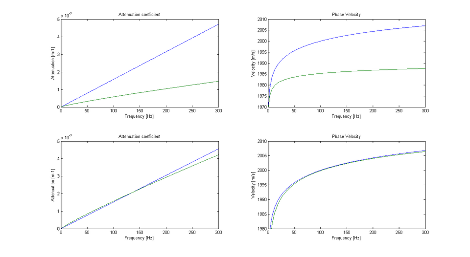
Studying the attenuation coefficient and phase velocity, and compare them with Kolskys Q model we have plotted the result on fig.1. The data for the models are taken from Ursin and Toverud.³

Data for the Kolsky model (blue):

upper: ${\displaystyle c_{r}=2000m/s,Q_{r}=100,w_{r}=2\pi 100}$

lower: ${\displaystyle c_{r}=2000m/s,Q_{r}=100,w_{r}=2\pi 100}$

Data for Azimis first model (green):

upper: ${\displaystyle c_{\infty }=2000m/s,a=2.5\times 10^{-6},\beta =0.155}$

lower: ${\displaystyle c_{\infty }=2065m/s,a=4.76\times 10^{-6},\beta =0.1}$

• 
  Azimis 1 model - the power law

Data for Azimis second model (green):

upper: ${\displaystyle c_{\infty }=2000m/s,a=2.5\times 10^{-6},a_{2}=1.6\times 10^{-3}}$

lower: ${\displaystyle c_{\infty }=2018m/s,a=2.86\times 10^{-6},a_{2}=1.51\times 10^{-4}}$

• 
  Fig.1.Attenuation - phase velocity Azimi's second and Kolsky model

References

- Wang, Yanghua (2008). Seismic inverse Q filtering. Blackwell Pub. ISBN 978-1-4051-8540-0.